Deriving Systems
Your programs print numbers at you all day. A duration in a log line, a benchmark summary, a p99 on a dashboard you scroll past. How many of them have you ever checked?
Not measured again. Checked: worked out what the number should have been, then looked to see whether the one on your screen was anywhere near it. Hardly anyone does, and it takes about ten seconds.
Here is what those ten seconds buy. Write a megabyte to a file, time the call, and it comes back in twenty-five microseconds. But a megabyte cannot cross a memory bus that quickly. At ten gigabytes a second it takes a hundred microseconds to move, and that is the floor for the fastest thing that could possibly have happened. Twenty-five is under the floor. So the work did not happen. Something you have done a thousand times just reported success, and it was not telling you the truth.
One division. No profiler, no flame graph, no afternoon gone.
This book is twelve of them. Nothing is looked up: each chapter opens with a measurement that cannot be true, spends a couple of pages on long division, and ends with one sentence worth remembering.
Start here: Twenty-Five Microseconds
Where that megabyte actually went.
There is a preface if you would rather know what you are holding first, and an introduction if you want the method stated plainly before you watch it used. Neither is required, and the first chapter assumes you skipped both.
Preface
This book began as an argument I was losing.
Somebody asked me why an fsync was slow, and I gave the answer
everyone gives, which is that it goes to the disk and disks are slow.
Then they asked how slow, and I did not know. I knew the shape of the
answer. I did not know the number, and it turned out that not knowing
the number meant I did not really know anything at all, because the
number was four orders of magnitude away from where my intuition had
quietly parked it.
So I started dividing. Not measuring: dividing. And what surprised me was how far you can get on a page of long division and a dozen constants you already half remember. Most of the questions I had been treating as research questions turned out to be arithmetic questions wearing a disguise, and the arithmetic took ten seconds.
That is the whole book. Twelve chapters of it.
Nothing is looked up
Where a number genuinely cannot be derived, and there are plenty of those, it arrives in a table labelled The Axioms, handed over explicitly. A cache line is 64 bytes because somebody once chose 64. There is no first-principles path to that, and pretending otherwise would be a lie in a book whose whole premise is not lying about where knowledge comes from.
Everything else is derived in front of you, including the parts where the derivation sets aside an answer I liked. I got things wrong writing this, and where the recovery taught more than the correction would have, I left the wrongness in and showed the recovery. Chapter 6 walks deliberately into a checksum that certifies its own failure.
Why bother, when you could just ask
Because you would get an answer, and an answer is not the same thing as judgment.
Ask a good model why your writes are slow and it will tell you about
page cache, write-back, and fsync, and every word of it will be true,
and you will be no better at the next question than you were at this
one. Knowledge really is one sentence away now. What is not one sentence
away is knowing which sentence to ask for, and that is a skill you build
only by doing the arithmetic yourself and occasionally being wrong by a
factor of a thousand in a way you remember for years.
I would rather hand you the habit than the facts. The facts are cheap and getting cheaper.
How to read it
Straight through, once. After that, not by rereading. Rereading a technical book feels productive and teaches almost nothing, because recognition is not recall and your brain is extremely willing to confuse the two.
Open the Rules Index instead. Fourteen sentences, one per rule, each linking back to the derivation that earned it. Pick one and try to rebuild the argument from the sentence alone. If you can, you have just proved it to yourself in a way no amount of rereading would. If you cannot, follow the link, and that failure is the most useful thing that will happen to you that day.
The Challenges page collects every question in the book with no answers attached, and that is permanent. Several cannot be answered from their own chapter at all and need something from a later one, or from outside the book entirely. Those are the good ones.
What it is not
Not a tuning manual: there is no list of flags to set. Not comprehensive: twelve chapters cannot cover storage, let alone storage and accelerators, and I chose depth on a few numbers over coverage of many. Not benchmarks: every experiment checks a ratio or an invariant rather than an absolute latency, because latencies belong to your hardware and ratios belong to the world.
When you want to stop reading and run something, the Experiments check the book's own claims on your machine, and The Course is twenty stages that build the inference engine Part IV derives. Commit to your number before you run either. That is the entire exercise, and it stings a little every time.
Introduction
Here is a scene you have been in.
Something is slower than it should be. Six people are in a room, or a thread, and within about ninety seconds somebody has opened a profiler. Within ten minutes there is a flame graph. Within a day there is a benchmark harness and a disagreement about statistical significance, and by the end of the week there is a great deal of beautiful data and no decision.
Nobody in that room did anything wrong. Every step was reasonable. But somewhere near the start, a question got asked that a single division would have settled in ten seconds, and instead of dividing, everybody instrumented.
I want to make the case that this is the normal failure, not the exceptional one, and that the fix is smaller and less impressive than you would like.
The claim
Most performance questions are settled by arithmetic you can do on paper.
Not all. Some genuinely need counters and careful statistics, and chapter 1 gives you a rule for telling which is which. But the ordinary case, the "why is this slow" that arrives on a Tuesday, is usually a question about which of two or three things dominates, and the things being compared are usually so far apart that a rough calculation separates them completely.
When candidates sit a thousand times apart, no amount of measurement noise closes the gap, and the stopwatch already knew the answer. Reaching for a profiler at that point is not rigour. It produces artifacts and consumes a week, and the week is the real cost.
What you actually need
Two things, and neither is a tool.
A dozen constants. Memory bandwidth, roughly. NVMe write bandwidth,
roughly. What an fsync costs. What a syscall costs. Cache line size.
The bandwidth and peak compute of whatever accelerator you own. Rough is
fine. Being within a factor of two is plenty when the candidates are a
thousand apart, and that is most of the time.
The willingness to commit to a number before you check. This is the part people skip, and skipping it is why measurement so often teaches nothing. If you write down "I think 300 microseconds" and it comes back at 5, you have learned something violent and permanent about your mental model. If you write down nothing and it comes back at 5, you nod and move on, and next year you will make the same mistake with the same confidence.
Prediction is what converts a measurement into a lesson. Without it you are collecting numbers, and numbers are not understanding.
The method
Every chapter in this book runs the same loop, and it is short enough to memorise.
Name the candidates. Where could the truth plausibly be? Two or three answers, stated plainly, before you have any attachment to which one wins.
Name the ratio between them, in the same breath. This is the move everything else rests on. Not "disk is slower than memory," which is a direction and cannot decide anything. How much slower. A question whose answers differ by a factor of a thousand splits the world and should be asked immediately. A question whose answers differ by less than two is a detail, and asking it early is procrastination wearing a lab coat.
Do the division. Take your dozen constants, work out what each candidate would cost if it were true, and compare that against what you actually measured.
See what survives. Usually one candidate is off by orders of magnitude and goes. Sometimes, and these are the best chapters, none of them survive, which tells you the question itself was malformed and you have just learned something you were not looking for.
That is it. There is nothing else in the bag.
Why the ratio, and not the answer
Because the ratio tells you whether the question was worth asking at all, and the answer does not.
If two candidates differ by 1.3×, then it does not much matter which is right, and any effort spent separating them is effort not spent on the thing that differs by 400×. Sorting your questions by the spread between their possible answers is the cheapest triage available, and almost nobody does it, because it feels like a step you can skip on the way to the real work.
It is the real work. The rest is division.
Why storage, and then GPUs
The book is in four parts. Parts II and III look like they belong to
different fields: one is about fsync and torn writes and crash
recovery, the other is about arithmetic intensity and KV caches and
tokens per second. Different decade, different hardware, different
vocabulary, different conferences.
They are here together on purpose.
If the method only worked on storage, it would be storage trivia dressed up as a principle. What makes it a method is that the same four steps, applied to a GPU nobody had when the storage chapters' ideas were invented, produce the same kind of answer. Group commit and GPU batching turn out to be the same trick. The floor test catches a fraudulent benchmark in chapter 1 and an unmodelled CPU cost in chapter 11. PagedAttention turns out to be virtual memory from 1962.
That is the actual claim of the book, and it is why the two halves sit next to each other rather than in two books.
What a rule is
Each chapter earns one, and each is a single sentence in a box. Chapter 1 is the exception and earns three, because it is about the method itself and the method has three moving parts.
They are short deliberately. A rule you cannot recall at eleven at night is not doing anything for you, and the test of whether you have learned one is not whether you agree with it but whether you can rebuild the derivation that produced it from the sentence alone.
Fourteen of them, collected in the Rules Index, which is the page to open when you have forgotten everything else.
The shape of a chapter
So you can navigate: an anomaly, a measurement that does not fit. Two candidates and the ratio between them. A table of axioms, the numbers handed over because they cannot be derived. The division. What that rules out, including at least one answer we liked. A picture. A rule. Four challenges with no answers. And a design note, which is the part where I stop deriving and tell you what I actually think.
Twelve times. Starting with a write that returns far too quickly to possibly have happened.
Twenty-Five Microseconds
Any sufficiently advanced measurement is indistinguishable from a lie.

I want to start with something you can do right now, without leaving this page. Write a megabyte to a file. Time the call. See what comes back.
On an ordinary machine, on an ordinary day, it comes back in about twenty-five microseconds.
Twenty-five microseconds is about how long it takes light to run seven and a half kilometres. Your megabyte did not go anywhere near that far.
Now, if you run that a hundred times, the number stops registering. It's small, the write worked, the test passed, and there's a whole afternoon of other work waiting. I have done exactly this and thought nothing of it. But twenty-five microseconds is the loudest thing that will happen to you all week, and this chapter is about learning to actually hear it.
We are not going to look anything up. By the end you will know exactly where that megabyte is sitting, and we will have gotten there with four numbers and some long division, which is honestly all this ever takes.
1.1 Two Candidates and a Missing Number
Let's start where everybody starts. Where could the data actually be?
Either it's still in memory, or it's out on the disk. That's a reasonable first cut. And the reflex that follows, the one I have had a hundred times, is to say disk is slower than memory and feel like some progress has been made.
It hasn't. Not really. That's a direction, and a direction cannot decide anything by itself. Both candidates are still standing, and we have no idea which way to lean, because we never asked the question that actually separates them:
How much slower?
This is the habit the whole book is built on, so it is worth saying plainly. When you name two possibilities, name the ratio between them in the same breath. The ratio is what tells you whether the question was worth asking at all.
1.2 The Axioms
Here is the part nobody quite says out loud. Some of this we cannot derive. Not because we aren't clever enough, but because there is nothing underneath it to derive from.
A cache line is 64 bytes because somebody, once, in a meeting, chose 64. DRAM latency is whatever physics and market economics happened to settle on between them. There is no first-principles path to either number. You just have to know it, the way you know a stop sign is red.
So let's take them as given. There is no shame in being handed a constant. The only real shame is needing to be handed the conclusion too.
| Path | Throughput |
|---|---|
| memory copy, single core | ~10 GB/s |
| NVMe SSD | ~2 GB/s |
| spinning disk | ~150 MB/s |
A dozen constants is fewer than most people carry for their own family's birthdays, and considerably more useful at two in the morning.
A dozen numbers roughly like these make up most of the toolkit. Twelve numbers. That's it. What we do with them is the entire skill.
1.3 Doing the Division
One megabyte, three plausible paths home.
Before you read on, write down what you think the answer is. I mean it, actually write it down. Not because the arithmetic is hard, but because committing to a value you might be wrong about is the whole exercise, and reading past this sentence without doing it is how you get the comfortable feeling of learning without any of the learning.
1 MB ÷  10 GB/s  =  100 µs     memory copy
1 MB ÷   2 GB/s  =  500 µs     NVMe
1 MB ÷ 150 MB/s  =  6.7 ms     spinning disk
Now let's put those next to the thing we actually measured.
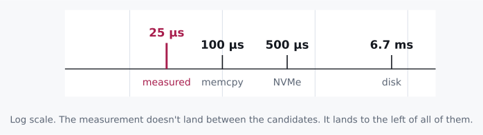
Sit with that a moment, because it is not the outcome anybody was set up to expect.
Twenty-five microseconds beats every option on the list. Every one. Including the option that never touches storage at all. So the conclusion is not "it must be in memory." The conclusion is much better than that: our list of candidates was wrong.
The ratio test did not just rank our candidates against each other. It caught that the question itself was malformed. Nobody told us we were buying that when we started dividing, and it is the most useful thing in the chapter.
Let me digress for a paragraph, because this rule has a family resemblance to something you have probably already lived through.
Years ago I watched somebody optimize a numerical loop and report a speedup of about four hundred times. Four hundred! Everyone was delighted. There was a graph. What had actually happened was that the result of the loop was never read, so the compiler noticed this and deleted the entire computation, and the benchmark was faithfully timing an empty program. The number was real. The measurement was honest. The work had simply not occurred.
The graph was beautiful. Somebody had put the four hundred in bold.
That is the same rule as the one in the box, wearing different clothes, and it is why I trust it more than almost anything else in this book. A result that is too good does not mean you won. It means you should go looking for the step that got skipped. Nobody moved a megabyte anywhere in twenty-five microseconds, and now we get to find out what got skipped.
1.4 Turning It On Our Own Answer
The textbook reflex here is page cache. The kernel took the bytes, parked them in its own memory, and returned without ever touching the device. Deferred write-back. It is clever, it is well documented, and it feels like an answer the instant you say it out loud.
So let's turn the floor test on it, exactly the way we would turn it on somebody else's claim.
Copying into page cache is still a memory copy. It is still a megabyte moving through a single core at ten gigabytes a second. That is 100 µs, a number we derived four paragraphs ago and now get to reuse for free.
Page cache is four times too slow to explain what we saw.
It does not survive contact with our own arithmetic. Not because we read something that contradicted it, not because an expert corrected us, but because numbers we already had in hand would not let it stand. That is a lovely way to be wrong. It costs nothing and it happens in ten seconds.
So the kernel never copied our data either. Which leaves something stranger and more interesting. Maybe nothing copied it at all.
1.5 Reading the Band
We have a floor. Now let's get a ceiling, coming at it from the other direction.
plain function call, off the stack  ~1–5 ns
null syscall (post-Spectre)         ~0.5–5 µs
1 MB memcpy                         ~100 µs
Twenty-five microseconds is five thousand times too slow for a bare function call, and four times too fast for a full DRAM-bandwidth copy. It is wedged between two floors, and the gap is narrow enough to mean something specific.
Twenty to fifty microseconds is the signature of a memcpy into a
buffer that is already hot in the CPU cache. L2 and L3 can move
data at 30–50 GB/s on a modern core, three to five times the
~10 GB/s you get when the destination lives in main memory. The
bytes never left your process. No syscall happened at all.
That is exactly what fwrite, BufWriter, and the default buffered
file API in most languages do. They keep your bytes in the process's
own memory and defer the syscall until there is enough to make the
trip worthwhile. At twenty-five microseconds, the floor test does
not reject this: 1 MB in 25 µs is roughly 40 GB/s, which is
comfortable L2/L3 cache bandwidth on a modern core.
So the explanation here is simpler than it first looked. The data
was copied, but only into a cache-hot userspace buffer sitting in
the CPU's own backyard. No kernel crossing, no device, no page cache.
Just a fast, local memcpy that the DRAM-bandwidth floor fails to
catch because the destination was never in DRAM.
What survives is the buffered copy: a memcpy into a cache-hot
userspace buffer that never crossed into the kernel.
And here is a detail I find genuinely delightful. Buffering explains plenty of fast returns, just smaller ones. Ask for four kilobytes instead of a megabyte and the copy costs well under a microsecond, and buffering becomes the likeliest answer in the room. The mechanism we land on depends on the size we asked about. Which is why the megabyte was in the question at all, and why "how fast is a write" is not a question that has an answer.
1.6 Resisting strace
Here is where most of us reach for a tool. I want you to resist for one more second, and ask what the tool would actually buy.
We are separating "no syscall," which is nanoseconds, from "syscall that enqueued," which is microseconds. Three orders of magnitude apart. No amount of measurement noise, scheduler jitter, or thermal drift closes a 1000× gap. The stopwatch already answered it.
Nobody has ever been criticized in a review for adding more instrumentation, which is most of what is wrong with reviews.
For the day you genuinely need them: strace -c counts syscalls,
perf trace times them. They are excellent tools and you should need
them far less often than you think.
1.7 So Where Is It
Four layers, in the order they would survive:
   YOUR PROCESS
 ┌──────────────────┐
 │ userspace buffer │  gone if your process crashes
 └──────────────────┘
          │  write()        ~1–5 µs
          ▼
   THE KERNEL
 ┌──────────────────┐
 │   page cache     │  survives a crash
 └──────────────────┘  DIES on power loss
          │  fsync()        ~100 µs – 10 ms
          ▼
   THE DEVICE
 ┌──────────────────┐
 │   drive cache    │  still volatile
 └──────────────────┘
          │
          ▼
 ┌──────────────────┐
 │  FLASH / PLATTER │  actually durable
 └──────────────────┘
At twenty-five microseconds, you are at level one. Not two. Not four.
Now, the names in that diagram are worth complaining about for a
moment. write() is the syscall that leaves userspace, which the
name rather undersells. Your data lands in page cache. And fsync() is
not "send it to the kernel," because it is already there. fsync is
what pushes it out of the kernel, toward the media.
write() does not write and fsync() does not send. Both names are older than I am and neither is going to be fixed now.
Most people know about fsync. What catches people off guard is
subtler, and it is the thing I would tattoo on a wall if I could: the
default path in nearly every file API stops one level short of durable,
and you have to opt into that last step on purpose. Closing a file
flushes userspace into the kernel. It does not sync.
Which sets up everything in Part II. That last arrow turns out to be expensive enough that entire database architectures exist for no reason other than to avoid taking it more often than they must.
experiments/01_write_latency.c writes
a megabyte four ways and prints each one against the floors above. Commit
to your four numbers before you run it. See Experiments.
Challenges
No answers here, on purpose. Re-deriving is the point. If you wanted to re-read, you would have the chat log.
-
You measure a 4 KB write at 900 ns. Which layer is it at, and what floor did you use to decide?
-
Your service acks a client immediately after
write()returns. Name the exact failure that loses acknowledged data, and the one that doesn't. -
A colleague says an optimization made the write path "three times faster." Using Rule 3, what's the first thing you'd ask, and what would make you reach for
perfinstead of a stopwatch? -
fsyncon NVMe costs ~100 µs.write()costs ~25 µs. Derive the maximum sustainable durable-write rate for a system that syncs once per request, and explain why real databases beat that number anyway.
Design Note: Procrastinating With Rigor
There is a specific failure mode that looks exactly like diligence, and I have fallen into it more than once.
You have a question. Instead of estimating an answer, you instrument. Flame graphs. Tracing. A benchmark harness. An argument with a colleague about statistical significance. Three days later you have beautiful data about something a single division would have settled in ten seconds, and the worst part is that everyone involved feels good about it, because it looked like the careful thing to do.
The tell is that you never wrote down what you expected.
Instrumentation without a prediction has no failure condition. Every result looks interesting. Nothing is surprising. And you learn remarkably little, because nothing you believed was ever put at risk. That is the whole trick of it: the process feels rigorous precisely because it cannot fail.
The discipline is cheap and it stings a little. Before you measure, commit to a number. Not "faster." Not "I expect an improvement." A number, with units, that you would be a little embarrassed to be wrong about by 10×.
Being wrong that way is what makes a lesson stick. I know which of my numbers were wrong by 10× and I do not remember a single one I got right.
The Ladder
Your test suite has never once lost power.
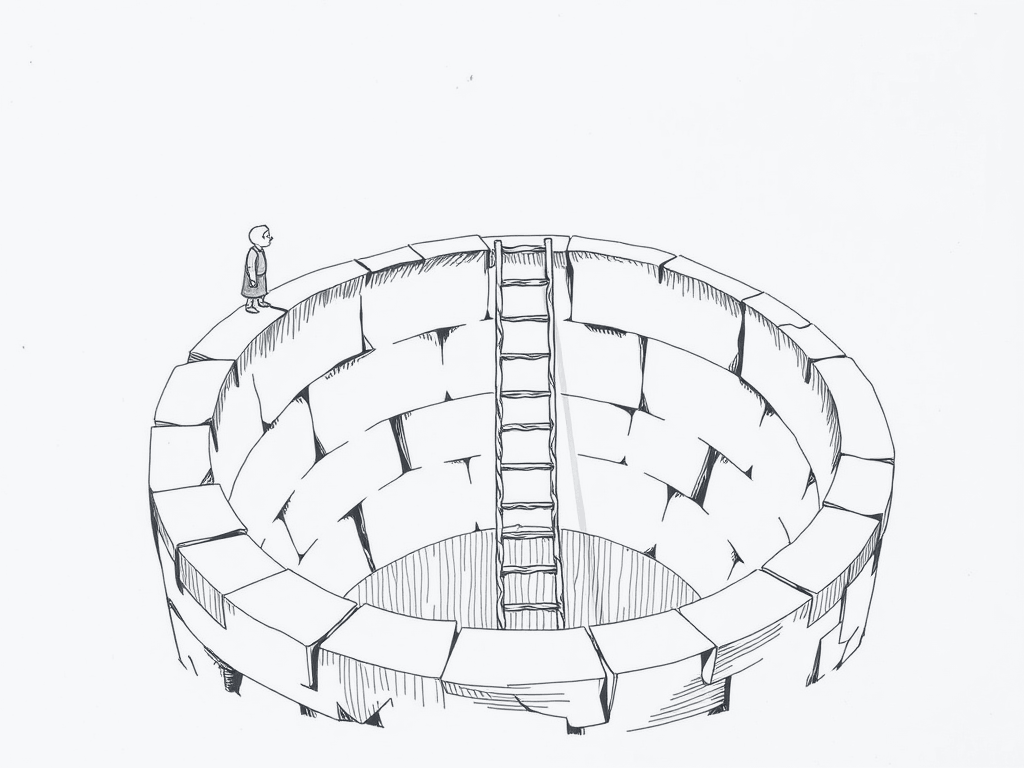
Let me tell you about a test that passed ten thousand times and proved nothing at all.
We build a crash-test harness for a write path we care about. It sends
kill -9 to the process mid-write, at a random byte offset, ten
thousand times. Zero bytes lost. Every single run. That feels
wonderful, so we ship it.
Six weeks later somebody runs the same workload through a power-fault rig instead. Not a signal: an actual switch that cuts the wall socket. It loses data on the very first try.
Ten thousand for ten thousand on one test. Zero for one on the other.
Ten thousand passes and a single failure, and the single failure is the only one that was asking the right question.
Now, that is not a flaky test. I want to be firm about this, because "flaky" is the word everyone reaches for and it is the wrong word, and reaching for it is how the afternoon gets wasted. Those are two different questions wearing the same costume, and the costume is the word "crash."
2.1 Two Candidates and a Missing Number
The natural reflex is to treat this as a probability problem. kill -9
failure is rare, power-loss failure is common, go collect more samples
and find the true rate.
Resist that. Ask Rule 1's question first: how much do the candidate answers actually differ?
And here the honest answer is that this is not a spread at all. It is a
category error. kill -9 removes a process. A power cut removes
power to the machine. Those are not two points on one axis. They are
different axes, and no quantity of extra sampling on one turns into
evidence about the other.
So the real question underneath "why did these two tests disagree" is a different one entirely: what does each failure actually destroy? Answer that, and both results stop being surprising at all.
2.2 The Axioms
There are four places a byte can live between write() and safe
forever. Each one is owned by something different, and ownership is the
thing that determines what can kill it.
| Layer | Owned by | Process death | Kernel panic | Power loss |
|---|---|---|---|---|
| Userspace buffer | Your process | No | No | No |
| Page cache | The kernel | Yes | No | No |
| Drive write cache | The device | Yes | Yes | Only with PLP* |
| Flash / platter | The device, non-volatile | Yes | Yes | Yes |
*PLP = power-loss protection, explained below.
That third row is the one nobody's intuition gets for free, and it is worth a digression, because it is where the money is.
The capacitor costs about forty cents. It is the difference between a drive that keeps its promises and one that merely makes them.
Consumer SSDs and spinning disks both carry a small volatile write cache on the device itself. Not in your process. Not in the kernel. Physically on the drive, after the data has already left the operating system entirely. The drive accepts your bytes into that cache and tells the kernel it is done, because from the drive's point of view it is done, and the drive has no opinion about your durability requirements.
Enterprise drives often ship power-loss protection: a capacitor, sized to hold enough charge to finish flushing that cache during the few milliseconds after somebody pulls the plug. Consumer drives usually do not. Same interface, same "write complete," same everything you can see from software.
So two drives can both report success and quietly disagree about whether that success survives a power cut, and the only difference between them is a component you cannot query, on a part of the machine your code never touches. I find that a little frightening, and I think you should too.
2.3 Doing the Division
There is arithmetic here, and it is not the arithmetic the harness looked like it was doing.
Ten thousand clean runs is a real statistical result. When you see zero failures in n trials, the ninety-five percent upper bound on the true failure rate is about 3/n. So the harness bought us a genuinely precise number:
     10,000 runs, 0 failures  ->  failure rate below 1 in 3,339
  1,000,000 runs, 0 failures  ->  failure rate below 1 in 333,809
That is defensible and it was not free. Somebody's machine ran for hours. Which makes it worth being exact about what it is a number about.
kill -9 deletes a process. A process owns row one. So every one of
those ten thousand trials was a trial of row one, and not one of them
was a trial of anything else. Run the division again with that column
added:
  trials that reached row 1        10,000
  trials that reached row 3             0

  95% bound, row 1 data loss   1 in 3,339
  95% bound, row 3 data loss          100%
Zero trials support no bound at all.
After ten thousand runs, our honest upper bound on losing acknowledged data to a power cut is one hundred percent. Exactly where it stood before anybody wrote the harness. Ten million runs would leave it at one hundred percent too, and so would ten billion, and this is the part I want you to feel: the number does not improve, ever, no matter how long you run it, because the experiment cannot reach the thing.
Statistics will cheerfully hand you a confidence interval on a question you never asked, and it will be a beautifully tight one.
The test was not flaky and it was not lucky. It was accurate to three significant figures about row one, while the data we were worried about lived three rows further down.
2.4 What This Rules Out
This retires a comfortable piece of folk wisdom: "we crash-test in CI, we're covered."
Covered against what, though? If the harness only ever sends SIGKILL,
it has validated exactly one row of the ladder, and it is the row that
was never in danger, because page cache does not care in the slightest
whether your process is still alive. The kernel is holding your bytes.
The kernel is fine. It watched your process die with total equanimity.
"We crash-test in CI" is a sentence about the CI. It is not a sentence about the crash.
The claim that needed testing was different: does an acknowledged
write survive losing the wall socket? Answering that requires reaching
row three or four. Which needs fsync(), which is the next chapter,
and a fault injector that removes power rather than signals: an IPMI
power-cycle, a managed PDU, a physical switch, somebody's foot.
Nothing short of that reaches the rows where the real risk lives.
2.5 The Pictorial
The table in 2.2 has the same information, but a table hides the thing that matters. Arrange it as a grid and the boundary jumps out: for each kind of failure there is one row where the crosses start, and that row is where your data stops being yours.
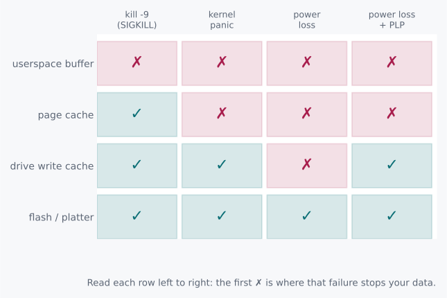
Chapter 1 got you to row one in twenty-five microseconds. The other three rows take the rest of the book.
Twenty-five microseconds put you on row one, back in chapter 1. The rest of this book is about what it costs, in time and in engineering, to walk down to row four on purpose. And about not fooling yourself into thinking you are already standing there.
Challenges
-
Your crash harness now uses
kill -9and reboots the VM (a cleanreboot, not a power cut) between runs. Which row does that combination actually validate, and which row does it still miss? -
A colleague proposes testing power loss by calling
echo b > /proc/sysrq-trigger(immediate reboot, no shutdown sequence) instead of physically cutting power. Where does that sit on the ladder: closer tokill -9or closer to a real power cut? Justify it from what each one actually destroys. -
An NVMe drive's spec sheet doesn't mention power-loss protection. What experiment would tell you whether it has it, without opening the case?
-
You have a fleet of machines behind a shared UPS. The UPS itself has a failure rate. Redraw the ladder's power-loss column as a function of UPS reliability. At what UPS failure rate does "no PLP on the drive" stop being a real risk in practice?
Design Note: Coverage Is a Claim About a Layer, Not a Count
"We have a crash test" and "we have crash coverage" are not the same sentence, and the gap between them is exactly the ladder.
A test count is seductive because it is a single number and it goes up.
Ten thousand runs feels like more assurance than one hundred, and in a
status meeting it reads like more assurance too. But the count only
starts to matter after you have established that the test can reach
the failure you are worried about. A million kill -9 runs against a
page-cache claim is a million data points about a question nobody
asked.
So before adding a zero to your run count, ask which row the test can possibly fail at. If the honest answer is row one, then more runs buy you a tighter confidence interval on a claim that was never keeping you up at night.
Better to redirect that effort at reaching row three, even if the run count goes down by three orders of magnitude as a result. Ten power cuts that reach the drive cache tell you something. Ten million signals that cannot reach it tell you the same thing they told you at run one, which is nothing.
The Barrier
fsync is not a save button. It is a purchase.
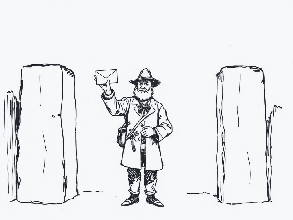
Here is a loop you can write in about a minute. Take an 8-byte counter. Append it to a file. Do that over and over.
In memory, that loop runs fifty million times a second. Now add one
call, fsync() after every append, and it runs two thousand times a
second.
Twenty-five thousand times slower. To persist eight bytes.
Not eight megabytes. Eight bytes. Hold that number next to the size for a moment, because something has gone badly wrong with our intuition about what we just bought.
If fsync were charging us for the data, eight bytes would be the
cheapest thing we could possibly ask it to do. So either the data is
enormously more expensive to move than we think, or we are paying for
something else entirely and the data is beside the point.
Those two possibilities are the whole chapter, so let's take them seriously one at a time.
3.1 Two Candidates and a Missing Number
The first candidate is the intuitive one. fsync is slow because it
moves our bytes to the device, and moving bytes takes time proportional
to how many bytes there are. Eight bytes is a small trip, but a trip to
a disk is a long way, and that is what we are paying for.
The second candidate says the byte count has nothing to do with it. We are being charged for something that would cost the same if we had handed over nothing at all.
Those two lead to opposite fixes, so it is worth an hour to tell them apart. And we can do better than an hour, because there is a division here that settles it in about ten seconds.
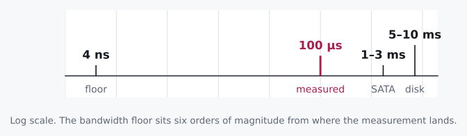
Name the ratio before you pick. At even a modest 2 GB/s of device bandwidth, eight bytes should cost:
8 B ÷ 2 GB/s ≈ 4 nanoseconds
We measured about 100 microseconds for that same call.
That is not a near miss. That is 25,000× over the bandwidth floor. The first candidate is not slightly wrong, or wrong in the details. It is wrong by more than four orders of magnitude, which is the kind of wrong you can see from orbit. Set it aside.
Being wrong by four orders of magnitude is oddly restful. There is no danger whatsoever that you were nearly right.
Which leaves candidate two, and a question we cannot answer by staring at it any harder: if we are not paying for bytes, what exactly are we paying for? For that we need some numbers.
3.2 The Axioms
We cannot derive what an fsync costs. It depends on a device, and a
device is a fact about the world rather than a consequence of anything.
So here are the three numbers, handed over, for the three kinds of
storage you are likely to be sitting on:
| Device | Typical fsync latency |
|---|---|
| NVMe SSD | ~100 µs |
| SATA SSD | ~1–3 ms |
| 7200 RPM spinning disk | ~5–10 ms |
Roughly a hundredfold spread top to bottom, which is worth knowing. But the spread is not the interesting part of that table, and if you take only one thing from it, take this instead.
Every one of those numbers stays nearly flat whether you sync 8 bytes or 8 kilobytes.
A cost that ignores a thousandfold change in the payload is trying to tell you something, and it is not being subtle about it.
That flatness is the whole tell. If a cost barely moves when you change the payload by a factor of a thousand, then the payload was never the dominant term. It was not even close to being the dominant term. You are paying for something else, and the size of your data is a rounding error on the bill.
So we are paying for an event rather than a quantity. The next question writes itself: what event?
3.3 Doing the Division
The answer is that fsync is not really a write at all. It is a
barrier.
It blocks until every write queued before it is provably sitting on non-volatile media. And it makes a second promise the name hides completely: a promise about order. Nothing after the barrier gets to be considered durable before everything ahead of it is.
Once you see it as a barrier rather than a save button, the flat cost stops being mysterious. You are not paying to move bytes. You are paying for a round trip: a request out to the device, a confirmation back, and a wait in between that no amount of shrinking your payload will shorten.
And that reframing immediately changes what we should do about it. Paying the barrier once for a batch of a thousand records, and paying it a thousand times for those same thousand records one at a time, are not remotely the same purchase. The first is one round trip. The second is a thousand of them, each one carrying almost nothing.
3.4 What This Rules Out
Take that rule seriously for a moment and notice what it costs us, because it is more than a tuning suggestion.
Twenty-five thousand times slower, for eight bytes. You could hand-deliver the eight bytes.
It rules out the intuition that durability is something you sprinkle on. "Just fsync after every write, to be safe." Safety is not the axis that scales badly here. Call count is. A service that fsyncs every record has chosen to pay a toll of 100 µs to 10 ms on every operation, however small, because the toll booth does not care what is in the trunk. It charges for the stop.
Now let me push on something we have been quietly treating as one thing, because I think it is really two, and separating them is what the next chapter is built on.
Durability and ordering are different purchases. You can imagine a system that needs its writes applied in order but does not need each one durable the instant it lands. You can imagine the reverse too: durability, with no opinion at all about relative order. Those are genuinely different requirements, and a careful engineer might well want to buy them separately.
fsync will not let you. It sells both, bundled, whether or not you
wanted the bundle.
Two guarantees, one price, and no itemized receipt.
And once you notice that, the design that follows is almost forced. Put only the thing that must be ordered and durable behind the barrier, and let everything else move lazily along behind it. That is chapter 4, and that is the entire idea. Before we get there, it is worth seeing the barrier drawn out, because the picture makes the waste obvious in a way the arithmetic does not.
3.5 The Pictorial
Here it is drawn out. Three records queued above the line, one crossing, and everything below it provably on the media:
 record 1 ─┐
 record 2 ─┤  queued, unordered w.r.t. the barrier
 record 3 ─┘
           │
     ══════╪══════  fsync()  ←  the barrier: one round trip,
           │                    ~100 µs – 10 ms, size-insensitive
           ▼
 [ record 1 | record 2 | record 3 ]  ← provably durable, in this order,
                                        only past this line
Three records behind the barrier, or three thousand, at the same price. Enjoy it. Very little else in this book is on offer.
That is the shape you want, and it costs one round trip no matter how many records are stacked above the line.
experiments/03_fsync_cost.c syncs
payloads from 8 B to 8 MB and prints how far the cost moved against how far
the size moved. Predict that ratio first. See Experiments.
Challenges
-
You batch 100 records behind one
fsyncinstead of syncing each individually. Using the NVMe number above, what's the best-case throughput improvement, and what would make the real improvement fall short of it? -
A teammate suggests using
fdatasyncinstead offsyncto skip metadata (mtime, size) updates. Under what circumstance does that optimization not actually save a barrier crossing? -
Two threads each call
fsyncon the same file at nearly the same time. Does the second call's cost look like a second full barrier, or something cheaper, and what would you measure to find out, per Rule 3? -
O_DIRECTwrites bypass the page cache entirely. Does that makefsyncunnecessary for durability? Name the specific claimfsyncmakes that a direct write, by itself, does not.
Design Note: The Bundle You Didn't Ask For
Every fsync call sells two things at once. This data is durable, and
everything before it happened first. Most of us only ever reach for it
because we want the first one, and we pay for the second without ever
noticing there was a second.
That would be fine if the second one were free. It is not. Ordering guarantees are precisely what turn a bandwidth-bound operation into a latency-bound one, because proving order means waiting for confirmation, and waiting is the exact opposite of throughput. You cannot pipeline a promise.
The systems that get this right unbundle it deliberately. They find the
one thing that genuinely needs the full barrier, and it is almost always
a small append-only log, and then they let everything downstream inherit
durability without ever calling fsync on its own behalf.
There is no trick in that. Nothing clever. They just declined to buy the bundle twice, which turns out to be a good deal of what separates a database from a program that writes files.
Write-Ahead
Never make a promise you cannot reconstruct.

I want to show you a bug that is worse than a lie, because everybody involved was telling the truth.
Suppose fsync() returns EIO. A real hardware write failure,
correctly detected, correctly surfaced. So we do the responsible thing:
we log it, and we retry the fsync.
The most dangerous error message is the one that says everything is fine.
It returns 0. Success.
The bytes it just claimed to have persisted were never written, and they never will be. The kernel is not lying to you. It is telling you the honest truth about the only attempt it still has any record of.
This was a real bug, found in PostgreSQL in 2018, and once you see why it happened, it changes what the phrase "handle the error" is even permitted to mean.
4.1 Two Candidates and a Missing Number
Before we decide what to do about that, we have to settle what actually happened, and there are two readings of it that lead somewhere very different.
The first: an fsync error behaves like any other I/O error. Log
it, back off, retry, and eventually it either succeeds or you escalate.
The second: retrying does nothing at all, because there is nothing left to retry.
This is not a ratio we can divide our way out of. It is a question about what the kernel does at the instant writeback fails, so let's just trace it through, slowly, because the answer is stranger than it looks.
A dirty page fails to reach the device. The kernel reports the error to
whoever calls fsync next, and it reports it once. Then it marks the
page clean and drops it.
Read that again. Not clean because it succeeded. Clean because the
kernel gave up and stopped tracking it as pending work. The data that
failed to write is now simply gone from the page cache. There is
nothing dirty left for a second fsync to flush.
Nobody lied. The kernel answered exactly the question it was asked, which was not the question anybody meant.
So the second call returns success. Honestly. From where it is standing, there is genuinely nothing left to do.
errseq_t) made sure
every open file description sees the error at least once, instead of the
first caller silently consuming it on everyone else's behalf. It did not
change the deeper fact underneath: the page is still discarded after one
failed writeback. Retry-until-success was broken before that fix, and it
is broken after it. The fix made the error easier to see. It did not
make the data come back.
4.2 The Axioms
There is no arithmetic to do here, which is unusual for this book. What we need instead are three facts about kernel behaviour, none of which you can reason your way to from first principles, and all three of which have to be true at once for the bug above to happen.
| Fact | What it means for us |
|---|---|
| A writeback failure marks the page clean and evicts it | The failed bytes are gone from the page cache, not "still pending" |
The error surfaces to fsync at most once per file description (post-4.13) | A second caller, or a second call, can see success on a page that never made it to disk |
| The kernel has no concept of "our" data, only dirty pages | It cannot retry on our behalf; it does not know what the bytes were for |
A backup on the same disk is not a backup. Everybody agrees with this, and roughly half of us keep one anyway.
Put those together and you get something that sounds almost harsh: an
fsync failure is not a transient fault to be retried. It is a
terminal event. The only sound response is to treat that data as lost
and rebuild it from somewhere the kernel did not just erase.
4.3 Doing the Division
That "independent, already-durable source" has a name. It is the write-ahead log, and the pattern that survives this failure mode is narrow and specific. Every clause in it is carrying weight:
1. write the record to the WAL          (userspace buffer)
2. fsync the WAL                        (the one barrier you pay for)
3. ACK the client                       ← the only line that matters
4. apply the change to the data pages   (lazily, async, whenever)
Steps 1 through 3 are the whole durability contract. Step 4 can happen a second later, a minute later, or after a crash and a replay, and it genuinely does not matter which, because if the crash arrives before step 4 finishes we do not need step 4's result. We need the WAL, and we already made certain that one thing was durable before we told anybody we were done.
The data pages, meanwhile, are allowed to be wrong. Half-written. Entirely missing. At any instant you care to inspect them.
That sounds reckless until you see why it is fine: they are derived state. They can be rebuilt. The WAL is the only object in this picture that cannot be reconstructed from anything else, and that is exactly why it is the one thing that gets the expensive, synchronous, ordered barrier we bought in chapter 3.
The data pages are allowed to be wrong. It takes a while to be comfortable writing that sentence down.
One barrier. On the one irreplaceable thing.
4.4 What This Rules Out
This rules out the natural instinct to spread fsync calls evenly
across everything that looks important.
Not all durable-looking writes are equally irreplaceable. A data page is
a cached, derivable projection of the log. Losing an unflushed data page
after a crash costs you a replay, which is to say it costs you some
seconds. Losing the log entry costs you the fact itself. There is no
second copy anywhere, and no amount of retrying a broken fsync brings
it back.
Now here is a question that looks entirely unrelated, and I promise it is the same question.
Why does PostgreSQL's torn-page protection (full_page_writes) take
its reference image from the in-memory buffer pool, and never by
re-reading the on-disk file it is trying to protect?
It would be so much simpler to read the file. The file is right there.
But the disk file is precisely the thing we do not trust. That is the entire premise of needing torn-page protection in the first place: a page write that crashes partway through leaves a sector-level mixture of old and new bytes. If our known-good reference came from reading that same file back, we would be verifying the disk against itself, and a corrupted page would cheerfully certify its own corruption.
Asking the suspect to vouch for the suspect. It passes every test you can think of, which is the trouble.
The buffer pool copy is the one version of that page our process actually validated. It is the only candidate in the room that is not circular.
Same rule as before, wearing different clothes: your recovery source has to be independent of the thing that failed.
4.5 The Pictorial
Four boxes and one arrow that matters. Watch where the acknowledgement sits, because everything in the design follows from its position:
 client request
        │
        ▼
 ┌──────────────┐   write()    ┌──────────────┐   fsync()    ┌──────────┐
 │  WAL record  │─────────────▶│  page cache  │─────────────▶│  device  │
 └──────────────┘              └──────────────┘              └──────────┘
                                                                        │
                                                         ACK client ◀───┘
                                                         (the only line
                                                           that matters)
        │
        ▼ (lazy, async, any time after the ACK)
 ┌──────────────┐
 │  data pages  │  ← derived. Can be rebuilt from the WAL.
 └──────────────┘     Never the thing we promised on.
Challenges
-
A junior engineer "fixes" the retry bug by calling
fsyncin a loop until it returns success three times in a row. Explain, from Rule 6, why this is no safer than calling it once. -
Your WAL fsync succeeds and you ACK the client. The process then crashes before applying the change to data pages. Walk through recovery. Where does the correct final state come from, and why doesn't it matter that step 4 never ran?
-
Suppose you moved the ACK to after the data pages are written instead of right after the WAL fsync. What does that change about your system's worst-case commit latency, and what do you gain for it?
-
full_page_writesdoubles WAL volume right after every checkpoint. Using Rule 5 from the previous chapter, propose a way to reduce that cost without weakening the torn-page guarantee.
Design Note: Design for the Failure You Can't Retry
Most error-handling advice quietly assumes failures are transient. Back off, retry, and eventually the world cooperates. That assumption is correct often enough that we stop noticing we are making it.
fsync breaks it quietly, which is far worse than breaking it loudly,
because the retry looks like it worked. It returns success. Your logs
show a transient error followed by a recovery. Everything about the
shape of it is reassuring, and every bit of that reassurance is false.
The lesson generalizes well past storage. Any time a failure silently discards the thing you were trying to protect, "retry the same operation" is not a recovery strategy. It is a way to convince yourself that you have one, which is strictly worse than knowing you do not, because the person who knows they have no recovery path goes and builds one.
The real fix is architectural, and it is not subtle: keep an independent, already-durable copy of anything you cannot afford to be wrong about, and make it durable before you promise anybody it is safe.
Write-ahead logging is not really a storage pattern, in the end. It is what "design for the failure you cannot retry" looks like once somebody draws it out on paper.
Group Commit
A constant that works at one load level is a bug waiting for load to change.
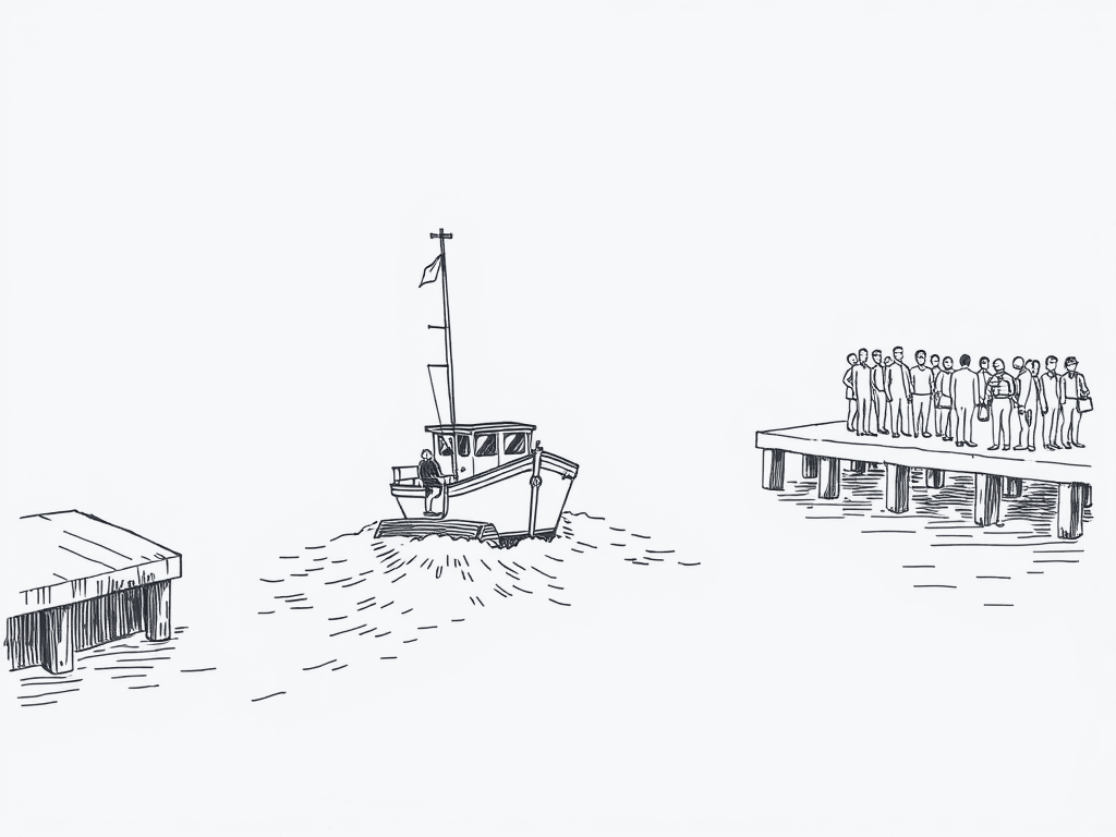
Say we have read chapter 3 and taken it seriously. Fsync-per-record was costing 25,000× what the bytes warranted, so we batch. Collect a thousand records, fsync once, acknowledge all of them together.
Under load, throughput jumps fifty-fold. We ship it. We are pleased with ourselves, and I think reasonably so.
A hundred seconds. Long enough to make a cup of tea while your database decides whether your write happened.
Then overnight, traffic drops to ten events a second. And the same code, unchanged, takes one hundred seconds to acknowledge a single write.
Now, nothing broke. I want to be careful about that, because the instinct is to go hunting for the bug. There is no bug. The arithmetic is exactly the arithmetic we should have expected: a thousand records arriving at ten per second takes a hundred seconds to fill the batch. We did not introduce a defect. We hard-coded a load level, and then the load politely changed on us.
5.1 Two Candidates and a Missing Number
So the constant was wrong. The interesting question is whether we should pick a better one or stop picking one, and those are genuinely different positions rather than degrees of the same one.
The first: pick a bigger fixed batch for throughput, a smaller one for latency, and tune the constant to match our traffic.
The second: stop picking a constant at all.
Name the ratio, because the ratio is the whole argument. A fixed batch of 1000 costs us:
at 100,000 events/sec:  1000 ÷ 100,000  =  10 ms  to fill    (fine)
at      10 events/sec:  1000 ÷      10  = 100  s  to fill    (not fine)
Ten million times worse. Same constant. Just a quieter night.
The constant did not change. The world did, and the constant had no way of finding out.
And that number is the argument against the first all by itself. There is no single value of N that is safe across a range that wide. Whatever you pick is correct at the traffic level you tuned it for and wrong by orders of magnitude everywhere else, and the place it is most wrong is the place nobody is watching, which is three in the morning.
5.2 The Axioms
One fact, and chapter 3 already handed it to us: an fsync round trip
costs about the same whether it carries one record or a thousand.
| Path | Cost per fsync |
|---|---|
| NVMe, one record | ~100 µs |
| NVMe, a thousand records | ~100 µs |
Look at that table for a second longer than it seems to deserve, because that equality is the entire opportunity.
Only one of these questions requires guessing about the future, which is a good reason to prefer the other one.
If a barrier crossing is nearly free per additional record, then the thing worth optimizing is not how many records we force ourselves to wait for. It is how many records happen to arrive during a crossing we are already paying for. Those are completely different questions, and only one of them requires us to guess about the future.
5.3 Doing the Division
So let's not set N at all. Let's set a rule instead.
When the in-flight fsync returns, immediately start the next one,
and sweep in everybody who arrived while the first was in flight.
t=0         fsync #1 issued (covers whatever's queued right now)
t=0..100µs  requests 2, 3, 4 arrive; they queue behind fsync #1
t=100µs     fsync #1 returns → ack 1; fsync #2 issued, covers {2,3,4}
t=100..??   whatever arrives now queues behind fsync #2
t=200µs     fsync #2 returns → ack 2,3,4; fsync #3 issued, covers {...}
Now watch what the batch size does. Nobody set it. It falls out of the arrival rate on its own.
At high load, dozens of requests pile up during one 100 µs window and ride across together, so we get the throughput win without ever naming a number. At low load, a request often finds nobody else queued at all, its "batch" is size one, and it waits exactly one fsync round trip. Not a hundred seconds. One round trip, which is the least it could possibly have waited.
The best batch size is the one nobody chose. There is a lesson in there about several other constants in your codebase.
That is the pleasing part. The scheme is not a compromise between the two cases. It is optimal at both ends, and it got there by refusing to answer a question it did not have to answer.
5.4 What This Rules Out
This rules out fixed-count and fixed-window batching as general answers. Not because either is wrong exactly, but because each one encodes an assumption about load that the adaptive version simply does not need to make. Fixed-count breaks at the low end. Fixed-window taxes everyone, always, including when nobody is waiting.
There is one wrinkle the naive adaptive version misses, and it is worth chasing down because it is the sort of thing that only shows up in production.
At moderate load, just under one arrival per fsync-latency window,
batches regress toward size one anyway, and we find ourselves firing an
fsync for very nearly every record. That is not a correctness
problem. Latency is fine. Throughput is fine. But it is the maximum
possible call rate, and on flash media, call rate correlates with write
amplification, and write amplification is measured in years off the
drive's life.
The fix is a small floor: hold the batch open for a minimum of roughly 200 µs, even if the in-flight fsync would have returned sooner. That caps how often the device gets hit, at the cost of a bounded, small, constant addition to latency.
The rejected idea comes back in the last act, behaving itself. This happens more often than the tidy version of engineering admits.
Which is the same trade as the fixed window we rejected two sections ago. Exactly the same trade. The difference is that here it is sized to be negligible instead of dominant, and I think that is worth saying out loud: the idea was never bad, it was just badly sized.
5.5 The Pictorial
The clearest way to see the difference is to put both policies on the same axis at two very different loads, and notice which one changes shape when the traffic does:
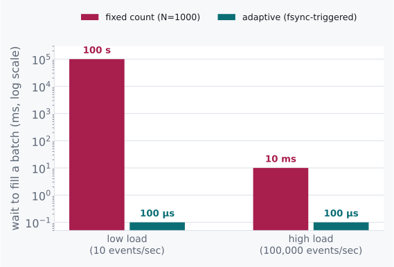
experiments/05_group_commit.c runs both
policies against real fsyncs at two arrival rates. Watch the adaptive batch
size change between them without anyone setting a number. See
Experiments.
Challenges
-
At exactly one arrival per fsync-latency window, adaptive batching's average batch size converges to what? Is that better or worse than fixed-count N=2 at the same load?
-
Your floor is 200 µs. Load spikes to 50,000 events/sec, well above what one fsync can drain in 200 µs. What happens to the queue, and does the floor still help or start hurting?
-
Two independent adaptive-batching writers share the same underlying log file. What has to be true about how they coordinate fsync calls for the scheme in 5.3 to still be correct?
-
Redraw the 5.1 arithmetic for a system with two tiers of durability need: some callers require the fsync ack, others are fine acking off the page cache. Does one adaptive batch still serve both, or do you need two?
Design Note: Tuning a Constant Is Postponing a Bug
Every hardcoded batch size, timeout, and thread-pool count is a bet that tomorrow's load looks like today's.
The bet is usually fine. That is what makes it dangerous. It holds through the tuning, through the load test, through the first six months in production, and then traffic has a bad night or a good launch or a regional failover doubles one region's share, and the constant does not fail loudly. That is the part I want to underline. It does not page anybody. It just quietly stops being the right answer, and the system keeps running, worse, until somebody eventually notices a hundred-second tail on a dashboard nobody was looking at.
The fix is not a better constant. It never is.
The fix is noticing which inputs to your formula are actually observable at runtime. Here it was one bit of information: is the fsync still in flight? That bit was sitting there the whole time, free, and it is strictly better than any number a human could have picked, because it is measured rather than assumed.
If you can replace a constant with a measurement the system already has in hand, that is not a nice-to-have. That is removing a bug before it happens, and those are the cheapest bugs you will ever fix.
Where the Truth Stops
Torn writes, CRC, and finding the edge of what survived.

Picture recovery scanning a log forward from the last checkpoint. It reaches the final record. There is a valid magic byte. There is a length field reading 200. And there are 200 bytes following it that parse cleanly into a well-formed record.
Every check passes. The record is fiction.
The first 71 bytes are real: they made it to disk before the crash. The remaining 129 are whatever happened to be occupying that block before this write ever started. And nothing about the record's structure tells us where the truth stops and the leftovers begin.
Corruption that looks like corruption is a gift. Nobody ever writes a postmortem about the bytes that looked wrong.
That is the thing I want you to sit with. Torn writes do not announce themselves. They do not arrive corrupted-looking. They look like data, because they are data. They are just somebody else's.
6.1 Two Candidates and a Missing Number
If structure cannot tell us where the record stops, we need to ask what can. There are two answers, and they differ in a way we can put a number on, which is the whole reason to prefer one.
The first: trust the framing. If the magic bytes check out and the length field points at something parseable, the record is real.
The second: do not trust framing at all. Verify the content.
The ratio that separates them is a coincidence rate, and it is a lopsided one. Structural framing has no floor on how often it accidentally looks right. A length field is two to four bytes. When a device has whole sectors of stale data sitting immediately behind your last good write, the odds of some short field reading as a plausible small number are not remotely negligible. They are not even small.
A 32-bit checksum has a known, tiny coincidence rate: roughly 1 in 4,294,967,296 that an altered message hashes to the same value by chance.
Four billion to one against, versus whatever the stale bytes happen to look like today. That is not a close call, and it is not a judgement call either.
6.2 The Axioms
So we want an arithmetic check rather than a structural one. Before we build it, here is what the standard one actually promises, because the guarantees are sharper than most people expect and the one gap in them is the whole of section 6.4.
| Property | Value |
|---|---|
| CRC-32 catches | all 1-bit and 2-bit errors, all odd-count bit errors, all burst errors ≤ 32 bits |
| CRC-32 misses (random corruption, non-adversarial) | ~1 in 2³² ≈ 4.3 billion |
| Computation | remainder of polynomial long division, in GF(2): XOR instead of subtract, no carries |
The mechanism here is arithmetic, not heuristic, and that distinction is the reason it does not share framing's blind spot. A CRC does not care whether the bytes look like a record. It has no opinion about what a record looks like. It only cares whether they divide down to the value the writer committed to before the crash.
6.3 Doing the Division
Long division, with subtraction swapped for XOR. You already know how to do this; you just did not know it had a Galois field in it.
I want to do this by hand. Not because you will ever need to, but because "it's just arithmetic" is the sort of phrase that stays abstract forever unless somebody makes you watch it happen once.
Take the message 1101011011 and the generator polynomial x⁴+x+1,
which is 10011, degree 4, so a 4-bit CRC. Append four zero bits and
divide, XOR-ing the generator in wherever the leading bit is 1:
  11010110110000    ← message with 4 zero bits appended
  10011              XOR (leading bit at pos 0 is 1)
  ───────────
  01001110110000
   10011             XOR (leading bit at pos 1 is 1)
   ───────────
  00000010110000                     (pos 2–5: leading bit 0, skip)
        10011        XOR (leading bit at pos 6 is 1)
        ───────────
  00000000101000
          10011       XOR (leading bit at pos 8 is 1)
          ───────────
  00000000001110

  remainder: 1110   ← the CRC
That is long division. The kind you learned at nine years old. The only difference is that subtraction has been replaced by XOR, so there are no carries and no borrowing, which if anything makes it easier than the version they taught you.
That 4-bit remainder ships alongside the message. On read-back we run the same division over the record including its stored remainder, and a clean write divides evenly and lands on zero.
Four billion to one is a comfortable margin. It is also a number you will meet in person if you write enough records.
A torn write, real bytes followed by stale ones, essentially never does. And the reason is worth stating plainly: the stale tail was not chosen to satisfy this particular division. It was chosen by whatever used to live on that block, months ago, by a process that had never heard of us.
6.4 What This Rules Out
This rules out "trust the length field" as a recovery strategy. Good.
But it also sets a trap for the checksum itself, and I want to walk into it deliberately, because it is the most satisfying mistake in this book.
Start the division register at zero, and an all-zero payload always produces an all-zero remainder.
Work it through with the long division above. If every bit of the message is zero, the leading bit is never 1, so the divisor never gets XORed in, not once. Zero goes in. Zero comes out. Every time.
Now, you might reasonably file that as a corner case not worth worrying about. I would like to talk you out of that, because zeroed blocks are one of the most common shapes a torn write takes. Plenty of filesystems and devices hand back zero-filled bytes for storage that was allocated but never written. This is not exotic. This is Tuesday.
Zero is the most popular number in computing, and every check you write should be asked what it does when handed a great many of them.
So picture the crash that leaves us a real header, followed by all zeros where the payload and the checksum should be. The zero-seeded CRC computes 0. It reads the stored trailer, which is also 0. It declares a match.
And there it is: corruption that looks valid, which is the exact failure this chapter opened with, sneaking back in through the one mechanism we built specifically to catch it. We did not fail to check. We checked, carefully, with real arithmetic, and the arithmetic said yes.
The fix is one line. Seed the register with a nonzero value before you
start. CRC-32's standard does exactly this, with 0xFFFFFFFF. An
all-zero message no longer produces an all-zero result, the degenerate
case that used to sail through now perturbs the register, and it gets
caught like anything else.
Thirty-two bits of careful mathematics, defeated by a block of nothing at all, and fixed by starting somewhere other than nothing.
One line. And you only ever find it by asking what your own check does on its worst input, rather than on a typical one.
6.5 The Pictorial
Here is what recovery sees when it walks the log and hits the crash. Two good records, then one that passes every structural test it has and fails the only test that counts:
 record 1 [ok, CRC matches]
 record 2 [ok, CRC matches]
 record 3 [header parses ✓] [71 real bytes][129 stale bytes] [CRC: NO MATCH]
                                           ▲
                                   the edge of truth
                               recovery stops replaying
                                      right here
experiments/06_crc_zero_seed.c shows
the all-zero record passing a zero-seeded check and failing a properly
seeded one. It is deterministic, so it prints the same thing on your
machine as on mine. See Experiments.
Challenges
-
A record's stored CRC matches, but the previous record in the log was itself torn and truncated the file mid-record. Does the matching CRC on record 3 tell you anything about whether record 3 is really the intended next record, or just something that happens to parse?
-
You upgrade from a 16-bit to a 32-bit checksum. Using the coincidence rate from 6.1, what's the new odds of an undetected corruption, and at what write rate would you expect to see one anyway over a year of operation?
-
CRC isn't cryptographically secure: an adversary who can choose the corrupted bytes can make the checksum match. Under what threat model does that matter for a crash-recovery log, and under what model doesn't it?
-
Design a scheme where the checksum itself could be torn (only part of the trailer made it to disk) but the record is still correctly rejected. What has to be true about where the checksum lives relative to the data it protects?
Design Note: A Passing Structural Check Is a Claim, Not Evidence
Length fields, magic bytes, and sentinel values all share a property that is easy to forget: they were written by the same process, at the same moment, as the data they are supposed to validate.
So if that write was torn, the framing can be torn right along with it. And a torn framing field does not reliably fail. Sometimes it just reads as a small, plausible, wrong number, and the parser has no way to know from the inside. The check and the thing being checked went down together, holding hands.
A checksum breaks that circularity because it is redundant on purpose. It encodes information that could only be true if the rest of the record is also intact. That redundancy is the entire value proposition, and it is the same argument that made PostgreSQL take its torn-page reference from the buffer pool rather than from the file it was protecting, back in chapter 4. Your verifier cannot come from inside the thing you are verifying.
It is worth noticing how rarely we apply this outside of storage. Any boundary where a producer and a much-later consumer have to agree about what actually happened in between has the same shape, and most of them are guarded by something that would fail exactly when it matters.
The Ridge
Arithmetic intensity, and the 99% idle GPU.

I want to show you a machine that costs thirty thousand dollars and spends nearly all of its life doing nothing at all.
It is an A100, and it can perform three hundred and twelve trillion arithmetic operations every second. We hand it a 7-billion-parameter model and ask for a single word. It computes for forty-five microseconds. Then it waits for seven milliseconds.
Thirty thousand dollars of silicon, idle 99.4% of the time. Even a landlord would be embarrassed.
Do the fraction. The thing is busy six-tenths of one percent of the time.
Now, when you first see a number like that, the natural thing to think is that somebody made a mistake. Sloppy code, a bad driver, an engineer who did not know what they were doing. I thought exactly that, the first time I saw it. It is the comfortable explanation, because it means somebody can go and fix it.
It is not a mistake. And what I want to show you is how you can prove that with arithmetic you can do on a napkin, and how, once you see why the machine is idle, you also see precisely what to do about it.
7.1 Two Candidates and a Missing Number
There are only two possibilities worth taking seriously here.
Either producing a word takes an enormous amount of arithmetic and the chip is straining to keep up. Or it takes hardly any arithmetic at all, and the chip is sitting there waiting on something that has nothing to do with arithmetic.
Those call for opposite remedies, so before anybody argues about which it is, let's just count. Generating one token from a 7B model, batch size one, costs roughly:
compute:  2 × 7×10⁹ params  ≈  14 GFLOP
memory:   7×10⁹ params × 2 bytes (fp16)  =  14 GB  read
Fourteen billion operations. Fourteen billion bytes.
One operation per byte moved.
One operation per byte. The most powerful chip in the building, being used as a very expensive way to read memory.
That ratio has a name, arithmetic intensity, and it is the only number this chapter needs in order to compute everything else.
7.2 The Axioms
One FLOP per byte is a fact about our workload. To know whether that is a lot or a little, we need the matching fact about the hardware, and that one we have to be handed. Two numbers off a spec sheet, and one ratio between them:
| Quantity | A100 (SXM, fp16) |
|---|---|
| Peak compute | ~312 TFLOP/s |
| Peak memory bandwidth | ~2 TB/s |
| Ridge point (compute ÷ bandwidth) | ~156 FLOP/byte |
The ridge point is where a workload stops being memory-bound and starts being compute-bound, on this specific piece of silicon.
Below it, the chip finishes its math faster than it can be fed, and sits idle waiting on the memory bus. Above it, the bus delivers data faster than the chip can chew through it, and the arithmetic units become the limit. It is a property of the hardware and nothing else. It does not know what you are running.
7.3 Doing the Division
Our workload sits at 1 FLOP/byte. The hardware's ridge is around 156. Let's line them up.
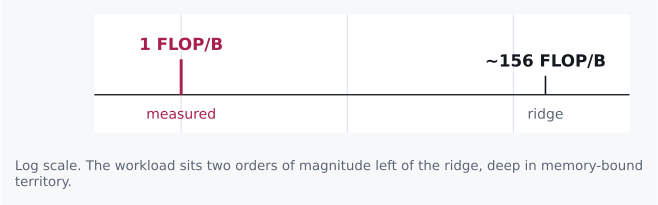
Now convert both halves into time, using the axioms:
compute time:  14 GFLOP ÷ 312 TFLOP/s  ≈  45 µs
memory time:   14 GB ÷ 2 TB/s          ≈  7 ms
Memory time is about 156× longer than compute time.
That is not a coincidence, and it is worth pausing on. That ratio is the ridge point, restated in seconds instead of FLOP per byte. The same number, wearing different units, arrived at from a completely different direction. When that happens you are usually onto something real.
The chip finishes its 14 GFLOP in 45 microseconds and then waits 6.95 milliseconds for the next byte of weight to show up.
7.4 What This Rules Out
This rules out the instinct to fix slow generation by buying a higher-TFLOPS card.
If your bottleneck sits 156× to the left of the ridge, tripling peak compute moves the ridge point further right and helps you not at all. You were never anywhere near the compute wall. You would be buying more of the thing you already have too much of, which is a wonderfully expensive way to change nothing.
There is always a bigger card, and it always comes with a graph showing how much bigger it is.
What would move the needle is more memory bandwidth. Or, and this is cheaper and much more interesting, changing the workload's arithmetic intensity itself.
Which is what this chapter has been building toward. At batch size one, we read the entire 14 GB of weights to compute one token's worth of math. At batch size 32, we read the same 14 GB once and compute thirty-two tokens' worth of math against it before the next byte has to arrive. The memory cost did not grow with batch size. The compute did.
It is worth doing that division in symbols, because the answer comes out cleaner than it has any right to. Call the parameter count N. Each weight is two bytes in fp16, and each weight takes part in exactly one multiply-and-add, which is two operations. At batch size B:
bytes moved  =  2 bytes/weight × N              =  2N
operations   =  2 ops/weight × N × B sequences  =  2NB

                 2NB
intensity  =  --------  =  B FLOP/byte
                  2N
The twos cancel. The parameter count cancels. What is left is the batch size itself.
When everything cancels and one variable is left standing, sit up. Nature is rarely that accommodating twice in a chapter.
Arithmetic intensity, for this workload, is B. Not approximately. Not in the limit. At batch 32 we sit at exactly 32 FLOP/byte, still under the ridge but far closer to it, and throughput scales almost for free on the way there.
That identity is the thing to carry out of this chapter. It turns the ridge point from a property of the silicon into a number you can type into a config file. A ridge of 156 FLOP/byte says, in plain language, run about 156 sequences at once. Every serving system in the world exposes that number as a tunable, and now you know what it is tuning against.
7.5 The Pictorial
Every serving framework has this knob. Most of the people turning it are doing so by feel, which is a shame, because it is just a division.
All of this fits on one chart, and it is worth learning to read because you will meet it again for the rest of your career. Arithmetic intensity runs along the bottom. The diagonal is what memory can feed you; the flat top is what the chip can compute. Where they meet is the ridge, and everything to the left of it is waiting:
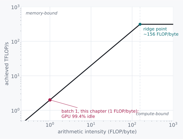
experiments-gpu/07_roofline.py measures
your own card's ridge point rather than quoting the A100's, then walks a batch
size toward it. A free Colab T4 is enough. Predict your ridge, and the percent
of peak you will get at batch 1, before you look. See
Experiments.
Challenges
-
Batch size 32 gets you to ~32 FLOP/byte, still left of the ridge. What batch size would this workload need to actually reach ~156 FLOP/byte, and what has to be true about your traffic for that batch to fill up without unacceptable latency?
-
A 13B model has roughly double the weight bytes and double the FLOPs per token of the 7B one. Does its ridge crossing point (in batch size) change, stay the same, or move, and in which direction?
-
Quantizing weights from fp16 to int8 halves the bytes read per token without changing the FLOP count much. Recompute arithmetic intensity at batch 1 under int8, and say whether this workload is any closer to the ridge.
-
Prefill (processing a whole prompt at once) replaces the matrix-vector multiply this chapter used with a matrix-matrix multiply, because many tokens' worth of activations move through the weights together instead of one at a time. Redo the 7.1 arithmetic for a 2048-token prefill pass: does the FLOP count grow with prompt length, does the byte count, and where does arithmetic intensity land relative to the ridge? (Nothing above answers this; you'll need to derive the matrix-matmul FLOP count yourself.)
Design Note: The Ridge Doesn't Care How You Feel About the GPU
"99.4% idle" reads like a scandal the first time you compute it, and the natural response is to go looking for somebody to blame. Bad kernels. An unoptimized runtime. A driver issue. Somebody upstream who did not care enough.
Usually none of that is true. The chip is idle because the arithmetic says it should be idle, and no amount of engineering effort inside a single forward pass, at batch size one, changes which side of the ridge you are standing on. You can rewrite that kernel with enormous skill and win nothing, and the failure will feel like your fault, and it will not be.
The lesson generalizes past GPUs. Any time you are tempted to profile harder to explain a bottleneck, check arithmetic intensity against the hardware's ridge point first. If you are two orders of magnitude to the left of it, the profiler is going to show you a chip waiting on memory no matter how you slice the flame graph, and the fix was never going to live inside the kernel you were about to spend a week on.
The Cache That Ate the Batch
512 KB per token, and why the field went where it went.

Put a 7B model on an 80 GB card and ask it to run 156 sequences at once.
It dies at 64.
Not 156. Sixty-four. Less than half, and it is not close. We did not tune a knob and miss by ten percent. The process died with an out-of-memory error, two and a half times short of the target.
That target was chapter 7's parting instruction, and it felt like a victory at the time. Batch 156 sequences together and we reach the A100's ridge point: the GPU stops idling, compute finally becomes the limit, everybody goes home happy. So we tried it, on the same model and the same card, and the card declined.
Sixty-four is not a tuning failure. It is an arithmetic result that nobody had got around to computing.
Something is spending memory that chapter 7 assumed was free.
8.1 Two Candidates and a Missing Number
Something is eating the difference, and there are two obvious suspects. One of them is a scheduling problem we could fix by being cleverer. The other is a cost we simply never counted.
The first: this is a scheduling problem. We are padding variable-length sequences to a common size, and the padding is eating the capacity.
The second: it is not padding at all. There is a second, growing memory cost that chapter 7 never priced.
Before we go hunting for padding bugs, it is worth checking the ratio. And the fastest way in is to ask what chapter 7 actually accounted for.
It accounted for exactly one thing living on that GPU: 14 GB of weights. It said nothing whatsoever about what accumulates during generation.
Now think about what has to accumulate. Every token already produced leaves behind a cached Key and Value tensor, kept around so the next token does not have to recompute attention over the entire prefix from scratch. That cache has a size. And it was completely absent from last chapter's arithmetic, not because anybody was careless, but because at batch size one, generating one token, there was nothing yet to accumulate.
8.2 The Axioms
For a 7B-class model (32 layers, 4096-dim hidden state, fp16):
| Quantity | Value |
|---|---|
| KV cache per token | 2 × 32 layers × 4096 dim × 2 bytes = 512 KB |
| KV cache per 2048-token sequence | 512 KB × 2048 = 1 GB |
| A100 total memory | 80 GB |
| Model weights (fp16, 7B) | 14 GB |
The factor of 2 is Key and Value: one tensor each, per layer, per token.
That is not an implementation detail you can shrink by being clever with your batching loop. I want to be firm about it, because it is the first thing people reach for. It is a per-token cost that accrues for as long as that token stays in context, for every sequence running concurrently, and no amount of scheduling makes it smaller.
A 2048-token conversation costs a gigabyte. The complete works of Shakespeare are about five megabytes.
Half a megabyte. Per word. Per conversation.
If you are used to thinking of a model as its weights, that is the number that will catch you out, and it caught me out too. The weights are the part that has a name and a download size. The cache is the part that decides how many people you can serve.
8.3 Doing the Division
With a number for what a token costs, the batch ceiling is one subtraction and one division. Take the card, remove the weights, and see how many one-gigabyte sequences fit in what is left:
memory budget for KV cache = 80 GB − 14 GB (weights) = 66 GB
sequences that fit          = 66 GB ÷ 1 GB/sequence  ≈ 66
Sixty-six. Before we account for activation memory, the CUDA context, and the other fixed overhead that eats a couple more gigabytes off the top, which is exactly how we land at the observed 64.
Somewhere there is a very tidy padding fix, thoroughly reviewed and merged with compliments, that bought absolutely nobody anything.
The KV cache arithmetic alone explains the shortfall. All of it. There is nothing left over for padding to be responsible for, and if we had gone hunting for padding bugs we would have found some, fixed them carefully, and moved the number by almost nothing.
8.4 What This Rules Out
This rules out the idea that chapter 7's ridge is reachable just by batching harder.
The ridge told us the compute-optimal batch size. This chapter shows the memory-optimal batch size is a harder ceiling sitting underneath it. We hit the KV wall at 64 before we got anywhere near the 156 the ridge wanted, and no amount of scheduling cleverness moves that. It is set by architecture and context length, and that is the end of it.
It also reframes what "add more GPU memory" actually buys. Linear headroom, at GPU prices, for a problem that feels quadratic from the inside. Every additional sequence costs another gigabyte for the whole time it is in flight, not once.
A gigabyte per conversation, for as long as the conversation lasts. Thinking out loud turns out to be an expensive habit.
So the field's answer was not bigger GPUs. It was making the 512 KB number itself smaller. And if you have ever wondered why half the acronyms in this corner of the field exist, this is where they come from: every one of them is an attack on that constant. Three moves, and you will meet all three.
- Multi- and Grouped-Query Attention (MQA/GQA): share Key and Value projections across several attention heads instead of computing a distinct KV pair for each. Divides the 512 KB directly by the sharing factor.
- KV cache quantization: store K and V in int8 or lower instead of fp16. The same lever as quantizing weights in chapter 7's challenge 3, pointed at the cache instead.
- PagedAttention: stop pre-allocating each sequence's cache for its worst-case length. Hand out fixed-size pages on demand, like virtual memory, so unused headroom in a short sequence is not locked away from a longer one running beside it.
Half the acronyms in this corner of the field are attacks on one constant. Once you know which constant, the reading list gets much shorter.
Every one of those attacks the 512 KB constant, or the waste around it. None of them touch the ridge point from chapter 7. Different wall, different tool, and that distinction is the whole reason these are two chapters instead of one.
8.5 The Pictorial
Two bars, one card. The top one is what we can actually run. The bottom one is what chapter 7 told us to run, drawn to the same scale so you can see exactly how far past the edge of the card it goes:
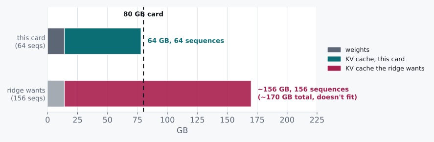
(Activation memory and other fixed overhead, a couple more gigabytes, are not shown. They are what pushes the real ceiling from 66 down to the observed 64.)
experiments-gpu/08_kv_cache.py allocates a
real KV cache and asks CUDA what it cost, instead of trusting the 512 KB
multiplication, and measures the exact factor GQA saves. A free Colab T4 is
enough. See Experiments.
Challenges
-
Grouped-Query Attention with a group size of 8 divides the KV cache per token by roughly 8. Recompute the batch ceiling on the same 80 GB card, and check it against the ridge point's target of ~156.
-
Sequences in a real batch don't all sit at 2048 tokens: some are 200 tokens long, some are 4000. Design a memory-accounting scheme for the 66 GB budget that handles this without falling back to "pad everyone to the max length." (This isn't fully answerable from this chapter alone; you'll need to think through what PagedAttention is actually doing under the hood.)
-
int8 KV quantization halves the 512 KB/token figure. Does it change the ridge point from chapter 7, or only the batch ceiling from this chapter? Be precise about which number moves and which doesn't.
-
A 70B model has roughly 10× the weights of the 7B one, but its KV cache per token doesn't scale by the same factor unless hidden dimension and layer count both scale linearly with parameters. Look up (or estimate from architecture) whether a real 70B-class model's KV-cache-per-token is closer to 5× or 10× the 7B figure, and redo the 80 GB budget.
Design Note: Two Walls Look Identical From the Outside
"Generation is slow" and "batch size is capped" arrive as the same complaint. Throughput is not what it should be. Somebody is unhappy.
Chapters 7 and 8 are proof that the identical complaint can have completely unrelated causes. One is a compute-versus-bandwidth ratio on the chip. The other is a bytes-versus-capacity ratio in memory. Neither diagnosis transfers to the other's fix, and neither one is visible from the complaint.
Buy a GPU with more TFLOPS and you have solved the wrong wall if you are capped by KV memory. Buy one with more memory and you have solved the wrong wall if you are capped by the ridge. Both purchases feel responsible. Both come with a graph. The only way to know which one you are actually against is to do both pieces of arithmetic, FLOP per byte against the ridge and bytes per token against the budget, before anybody spends money on either.
That is more or less the whole book in a sentence: two numbers that do not fit are two different chapters, and they very rarely share a fix.
The Slot That Waited
Eight sequences in flight, and one of them doing all the work.
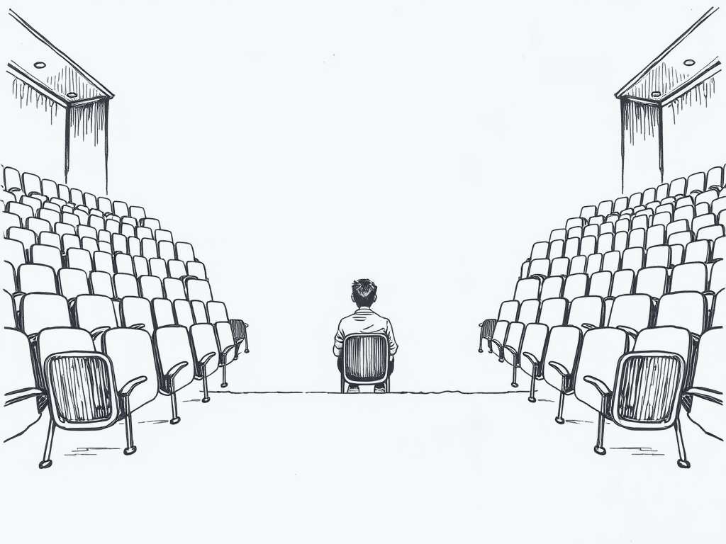
Size the batch at 64, fill every slot, and go and look at the throughput counter with some optimism.
It reads like a batch of sixteen.
Now, everything checks out. Every slot is occupied. Memory is full. The scheduler reports 64 live sequences and nothing is queued. And we are getting a quarter of the tokens per second that chapter 7's arithmetic promised for a batch that size.
The 64 was not a guess, incidentally. It is chapter 8's number: on an 80 GB card the KV cache holds about that many, so we took it at its word and filled every slot it would give us.
Nothing in the last two chapters explains a factor of four. So let's go find it.
9.1 Candidates and the Ratio
Two explanations fit what we are seeing, and it is worth separating them carefully, because one of them is a bug and the other is a decision we made on purpose without noticing.
The first: chapter 8's budget was optimistic. Activations, workspace and fragmentation ate more than the couple of gigabytes we waved at, so we are not really running 64 sequences. We are running sixteen and misreporting it.
The second: all 64 slots really are occupied, and most of them are occupied by sequences that finished a while ago.
It is worth separating those carefully, because they have opposite fixes. The first is a memory-accounting bug, and you solve it by measuring more carefully. The second is not a bug at all. It is a consequence of how we decided to schedule, and no amount of careful measurement will shift it by a single token.
9.2 The Axioms
Here is the thing chapters 7 and 8 never priced: sequences do not finish together.
Two of them, sitting side by side in the same batch, can differ in output length by two orders of magnitude, and neither one is unusual.
| Quantity | Value |
|---|---|
| "What is 2+2?" | ~5 output tokens |
| "Explain the CAP theorem" | ~400 output tokens |
| Ratio between them | ~80× |
| A batch, once launched, runs until | its slowest member finishes |
That last row is doing all the damage, and I want to point at it directly, because it is a choice dressed up as a law.
"What is 2+2?" and "Explain the CAP theorem" are billed at the same rate, and one of them is subsidising the other rather heavily.
We launch a batch. We run it to completion. We launch the next one. That is the obvious way to write the loop. It is how you would write it on a whiteboard, it is how every framework wrote it the first time, and there is nothing wrong with it except what it costs.
9.3 Doing the Division
Take eight requests with a spread any real service would call a quiet afternoon, and count the slot-steps we bought against the slot-steps we used. A slot-step is one sequence occupying one batch slot for one forward pass. It is the atomic unit of the thing we are actually paying for.
output lengths        =  5, 8, 6, 120, 7, 9, 6, 11
batch runs for        =  max(lengths)          =  120 steps
slot-steps purchased  =  8 slots × 120 steps   =  960
slot-steps used       =  5+8+6+120+7+9+6+11    =  172

occupancy  =  172 / 960  =  18%
You bought eight seats and one passenger. The airline model, applied to compute.
Eighteen percent.
We provisioned a batch of eight and got the throughput of roughly one and a half. Scale the same distribution up to 64 slots and the shortfall is the factor of four we measured, with room to spare.
If you carry one number out of this chapter, carry occupancy rather than batch size. Batch size is what you configured. Occupancy is what you bought, and nobody puts it on a dashboard.
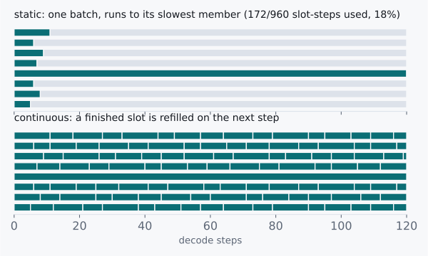
Look at the top half of that picture for a moment. Seven of the eight lanes go dark inside the first eleven steps and then just sit there, dark, for another hundred and nine, while one long sequence grinds to the end.
Batch size is what you configured. Occupancy is what you bought. Only one of them is on the dashboard, and it is the wrong one.
The slots did not fail. They finished. And then they waited, because we never built them a way to leave.
9.4 What This Rules Out
This rules out the memory-accounting candidate, and it rules it out cleanly, because the arithmetic above never mentions bytes. Not once.
You can hand the scheduler a perfectly measured 64-sequence budget and still get 18% occupancy, because the waste is in time, not space. Every fix aimed at memory (a tighter budget, less fragmentation, a bigger card) leaves that number exactly where it is.
It also rules out the reflex to blame padding, which is where most people go first, myself included.
Padding is real. Shorter prompts get padded up to the longest one in the batch, and those padded positions cost attention work. But padding is bounded by the spread in prompt lengths within a single step, which is a small constant. What we just measured is bounded by the spread in output lengths across the batch's whole lifetime, which is 80×. Those are not the same problem and they are nowhere near the same size, and if you spend a week on the first one you will move the second one by nothing.
Padding is the wrong suspect, and it has the enormous advantage of being easy to arrest.
What survives is the second, and the fix falls straight out of it. If the loss comes from a finished sequence holding a slot, then let it go. After every forward pass, ask which sequences emitted an end-of-sequence token, evict them, and admit whatever is queued into the space they left behind.
The batch stops being a fixed group of requests that start and end together, and becomes a running set that sequences join and leave continuously.
The idea comes from Orca (OSDI '22), where it is called iteration-level scheduling, and it is the largest single throughput win in modern inference serving. Not because it makes any kernel faster. Not one kernel changed. Because it stops us renting slots to sequences that finished their work and had nowhere to go.
9.5 The Pictorial
The mechanism fits in a loop short enough to read in one breath:
every forward pass:
    admit    while len(running) < max_seqs and queue is not empty:
                 prefill the next request, splice it into the batch
    harvest  record each running sequence's newest token
    evict    drop the ones that hit EOS or their token budget
    forward  one single-token pass over whatever survived
The largest throughput win in modern inference serving is four lines long and swaps the order of two of them.
Four steps. And the order of the middle two is the entire chapter. Evict before the forward pass and a finished sequence costs you nothing. Evict after it, or at the end of the batch like we used to, and you are back at eighteen percent.
Challenges
-
The loop above evicts finished sequences before the forward pass. Work out what happens to a request's output if you evict after it instead, and say precisely which token goes missing.
-
Admitting a new request means prefilling its prompt and splicing that prompt's KV into a batch whose sequences are all at different lengths. Sketch the tensor operations that requires, and estimate how much copying happens per admission. Then say what the copy cost is proportional to, and why that makes admission expensive at exactly the moment you want it to be cheap.
-
With the loop above and a 64-slot budget, what workload would still produce low occupancy? Describe the output-length distribution that defeats iteration-level scheduling, and say whether you think it occurs in practice.
-
A request arrives while the batch is full. Iteration-level scheduling says it waits for a slot. Chapter 8 says slots are bounded by KV memory, not by a count. Design the admission rule that decides whether a newly arrived request can start, given that you do not know how long it will run. (Nothing above answers this; the next chapter changes the memory model underneath it, which changes the answer.)
Design Note: The Cheapest Optimizations Are Refusals
Nothing in this chapter made anything faster.
I want to be precise about that, because it is easy to skim past. No kernel changed. No byte moved sooner. No arithmetic got cheaper. We found a place where the system was doing work it did not have to do, and we stopped doing it.
That is worth noticing, because it is the pattern behind most of the large wins in this book. Group commit did not make fsync faster, it stopped calling it once per writer. Write-ahead logging did not make the disk quicker, it stopped waiting on data pages before acknowledging. Here we did not make decoding faster, we stopped renting slots to sequences that had already gone home.
The engineering instinct, faced with a throughput number that is four times too low, is to go looking for something to speed up. That instinct is strong and it feels productive and it is usually the second best thing to do.
Spend an hour first on the less flattering question: what is this system doing that it does not need to do at all? The answer tends to be cheaper to implement and larger in effect than whatever you were about to optimize, and it has the rare and pleasant property that the code gets shorter.
A Page Table for Tokens
The KV cache we paid for, and the KV cache we used.

Go and measure what a real service actually produces. The mean request runs to about 350 tokens. Not 2048. Three hundred and fifty.
That is a sixth of the length the last two chapters budgeted for, so the card ought to hold something in the neighbourhood of four hundred sequences.
It holds 66.
A budget that cannot go down is not a budget. It is a bill.
It held 66 back when requests averaged 2048 tokens, and it holds 66 now that they average 350. The budget did not notice that the work got smaller, and I find that a genuinely strange thing for a budget to do.
Those figures are chapter 8's: 512 KB per token, 1 GB per 2048-token sequence, and 66 GB of free memory holding about 66 of them. Chapter 9 then taught those 66 slots to release themselves the moment they finish. Neither chapter ever priced a sequence that stops early.
10.1 Candidates and the Ratio
Either the number is right and our expectation was wrong, or the number is wrong and something is being wasted. Both are respectable positions until we do the arithmetic.
The first: 512 KB per token is simply what it costs, the requests are longer than we think, and 66 is the honest answer.
The second: we are paying for tokens that do not exist.
The ratio between those is the ratio between 2048 and 350, which is about six. That is well past the point where it is worth an hour to find out which one is true, and the two answers point at completely different purchases. One says buy memory. The other says stop wasting the memory you already have.
10.2 The Axioms
The reason the budget cannot notice that requests got shorter is that it is committed before the first token is ever generated.
| Quantity | Value |
|---|---|
| KV cache per token, 7B fp16 | 512 KB |
| Maximum context we must support | 2048 tokens |
| Reserved per sequence at admission | 2048 × 512 KB = 1 GB |
| Mean tokens actually generated | ~350 |
| Actually used per sequence | 350 × 512 KB = 175 MB |
That middle row is the axiom, and like chapter 9's it is a choice wearing the costume of a law. Let me take it apart, because three separate facts conspire here and none of them looks like a problem on its own.
A sequence's KV cache has to be contiguous, because attention strides through it as a single tensor. It has to be allocated before generation starts, because we cannot move it afterwards without invalidating every pointer into it. And its final size is unknowable at admission, because the model decides when to stop and it has not decided yet.
Reserved for a conversation nobody had, in the most expensive memory anybody sells.
Three reasonable facts. Put them together and the allocator's hand is forced: reserve the worst case, or risk running out mid-sequence with nowhere to grow.
10.3 Doing the Division
So put the reservation next to the reality. One line for what every sequence is charged at admission, one for what it turns out to need, and the gap between them is the whole problem:
reserved per sequence  =  2048 tokens × 512 KB  =  1024 MB
used per sequence      =   350 tokens × 512 KB  =   175 MB

waste  =  1 − 350/2048  =  83%
Eighty-three percent of the most expensive memory in the building, held against tokens that were never generated and never will be.
The vLLM paper measured this across real serving traces and put the figure between 60% and 80%, so our 83% is the high end of an entirely ordinary range rather than some pathological case I constructed to make a point.
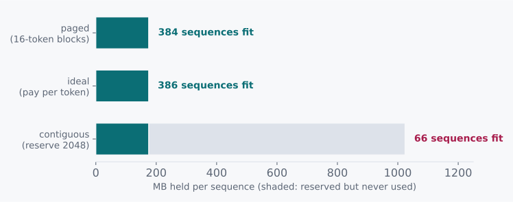
And now, if you squint at the problem rather than at the vocabulary, the answer becomes visible. Because this is not a new problem.
The Atlas computer shipped virtual memory in 1962. The paper reinventing it for attention came out sixty-one years later.
A resource that must appear contiguous to whoever is using it, whose final size is unknown when you allocate it, handed out to many processes at once. That is the problem operating systems solved in 1961. And the answer then was to stop making physical contiguity a requirement at all.
So: chop the KV cache into fixed-size blocks, sixteen tokens each. Give every sequence a small array mapping its logical block index to whichever physical block it happened to get. Allocate a block when the sequence grows into it, and not one step sooner.
blocks needed for 350 tokens  =  ceil(350 / 16)  =  22 blocks
allocated                     =  22 × 16 tokens  =  352 tokens
waste                         =  2 tokens
Two tokens. Against 1698 under reservation.
The waste is now bounded by the block size instead of by the context limit, which is to say it is bounded by a number we chose rather than a number the model chose. That is the whole difference, and it is worth more than it sounds.
10.4 What This Rules Out
This rules out buying memory, on economics rather than principle.
A card with twice the memory takes our 66 sequences to 132, at GPU prices, while leaving 83% of both cards idle. Fixing the allocator gets us to 384 on the card we already own. When a resource is 83% wasted, the return on buying more of it is seventeen cents on the dollar, and that ratio holds no matter how much of it you buy. You cannot purchase your way out of a waste fraction.
Seventeen cents on the dollar, and the ratio is politely indifferent to how many dollars you bring.
It also rules out a subtler instinct, which is to shrink the context limit. Dropping the maximum from 2048 to 512 genuinely would cut the reservation by four. It would also break every request that needed more than 512 tokens, which is a product decision smuggled into a memory optimization, and those are the worst kind of decision because nobody is in the room to object. Paging gets the same memory back without ever telling a user their conversation is too long.
What survives is the indirection, and it pays a second dividend that has nothing to do with waste.
Once a sequence's cache is a list of block pointers instead of a contiguous range, two sequences can point at the same block. A prompt that many requests share, the system prompt every conversation starts with, gets computed once and pointed at by all of them. Refcount the blocks, copy on write when a sequence diverges, and prefix sharing falls out of the very same table we built to fix fragmentation.
You go in to fix fragmentation and come out holding prefix sharing. Nobody planned that, and everybody takes the credit.
That is the sign of a good structure, incidentally. You build it for one reason and it hands you a second thing you were not asking for.
10.5 The Pictorial
Two sequences, sixteen tokens to a block, sharing a system prompt they both begin with:
  seq A logical:  [ 0 ][ 1 ][ 2 ][ 3 ]
  block table A:    7    3    9   12
                    |    |    \    \
  physical pool:  [ 7 ][ 3 ][ 9 ][12 ][ 4 ][ 1 ] ...
                    |    |    /
  block table B:    7    3    4
  seq B logical:  [ 0 ][ 1 ][ 2 ]

  blocks 7 and 3 are the shared prompt: one copy, refcount 2
  logical order is contiguous; physical order is whatever was free
The left half of each sequence is literally the same memory. Neither sequence can tell, and neither one ever sees a physical address.
Challenges
-
Block size 16 is the standard default. Compute the average internal fragmentation per sequence at block sizes 1, 16 and 256, then say what goes wrong at each end. One of the two failure modes is not about memory at all.
-
Chapter 9's challenge 4 asked how to decide whether a newly arrived request can be admitted. Paging changes the answer: a sequence now needs one block to start rather than 1 GB. Write the admission rule, and then find the failure it introduces, which is that a sequence admitted cheaply can run out of blocks halfway through generating.
-
Two sequences share a block by refcount. One of them generates a token that lands in that shared block. Describe exactly what must happen, in what order, and what goes wrong if the refcount is decremented after the copy instead of before.
-
Prefix sharing needs to recognise that two requests begin with the same tokens. Hashing each block's contents is the obvious approach. Work out why hashing a block's own tokens alone is not enough, and what else has to go into the hash. (The failure this prevents is a correctness bug and a privacy bug at the same time.)
Design Note: The Answer Was Sixty Years Old
PagedAttention is a 2023 paper about a 2023 problem, and its central idea is virtual memory, which shipped in the Atlas computer in 1962.
The mapping is not an analogy the paper reaches for in the discussion
section to sound erudite. It is the design. Blocks are pages. Block
tables are page tables. Sharing is fork. Divergence is
copy-on-write. Running out is a page fault, handled by eviction.
There is something in that worth more than the specific trick.
The KV cache problem arrived looking like a machine learning problem, and it was wearing all the machine learning clothes: attention, tokens, transformers, hardware nobody had five years earlier. Solve it as a machine learning problem and you get machine learning answers, and the field did try those first. Smaller caches. Shorter contexts. Cleverer padding. All reasonable. All small.
But describe it in its own terms and it is a memory allocator with unpredictable per-client growth against a hard ceiling. That description has sixty years of prior work bolted to it, and the prior work is better than anything you or I would derive from scratch in a quarter, because a great many careful people already spent their careers on it.
The skill being exercised there is not knowing about paging. Most working engineers know about paging. It is noticing, while surrounded by transformer vocabulary, that the thing in front of you has a shape you have seen somewhere before.
Below the Floor
Two hundred and eighty launches, and the bus waiting through all of them.
A 0.6B model in bf16. 1.19 GB of weights, on a card whose streaming bandwidth measures 380 GB/s. Every number small enough to hold in your head, which is the only reason to use a model this size.
roofline floor  =  1.19 GB ÷ 380 GB/s  =  3.13 ms/token
measured        =                         7.80 ms/token
Two and a half times the floor.
That floor is chapter 7's promise, presented for payment. If decoding is memory-bound, then the time to make a token should be the time it takes to drag the weights across the bus. Nothing more. Nothing else is on the critical path. Promises like that are checkable, and I think you should check them, especially the ones you like.
Check the promises you like best. They are the ones nobody else is going to check for you.
The card is achieving 153 GB/s out of the 380 it demonstrably has, which is forty percent of a bus chapter 7 said should be saturated. Somewhere inside every single token, four and a half milliseconds are going somewhere that is not the memory bus, on a workload we have spent two chapters calling memory-bound.
11.1 Candidates and the Ratio
There are two ways to explain a measurement that misses its floor, and they point in opposite directions: either the floor is wrong, or our account of where the time goes is incomplete.
The first: the 380 GB/s figure is a streaming-copy number, and the weight reads in a real forward pass have an access pattern that cannot reach it. Real achievable bandwidth here is nearer 153 GB/s, and the floor was wrong from the start.
The second: the bus really does deliver 380 GB/s, and the extra 4.67 ms is time when nothing is being read at all.
Chapter 1 handed us the tool for exactly this shape of question, and it is worth going back for it. The floor test says a measurement that beats a theoretical floor means the work did not happen.
This is that same rule, looked at from the other end. A measurement that misses a floor by 2.5× means work happened that we were not counting. Either the floor is wrong, or our picture of what the machine is doing has somebody missing from it. Those are our two candidates, and the arithmetic can tell them apart without us guessing.
11.2 The Axioms
To tell those apart we need to know what the machine is made of, and in particular we need one number that neither of the previous two chapters ever asked for. The first four rows below are about the model and the card. The fifth is about something else entirely:
| Quantity | Value |
|---|---|
| Model weights, 0.6B bf16 | 1.19 GB |
| Measured streaming bandwidth | 380 GB/s |
| Transformer layers | 28 |
| GPU operations per layer (attention, MLP, norms) | ~10 |
| CPU cost to dispatch one operation, eager PyTorch | 5–20 µs |
That last row is the one chapters 7 and 8 never mentioned, and notice that it is not a GPU number at all.
Every kernel that runs on that card was put there by the host. A Python call, a dispatch through the framework, a driver call that enqueues work on a stream. The GPU does not read its own program and decide what to do next. Something on the CPU has to hand it each piece, one at a time, all day long.
11.3 Doing the Division
So let's count the handoffs in one token.
operations per token  =  28 layers × ~10 ops  =  ~280 launches

unaccounted time      =  7.80 ms − 3.13 ms    =  4.67 ms
per launch            =  4.67 ms ÷ 280        =  ~17 µs
Two hundred and eighty times per token, a CPU says go, and a GPU that could have started already waits to be told.
Seventeen microseconds per operation, which sits comfortably inside the 5 to 20 µs the axiom table gives for eager dispatch.
The gap is not some mystery quantity we have to attribute on faith. It is 280 individual acts of a CPU telling a GPU what to do next, each one costing about what a Python-dispatched kernel launch costs, and together they account for the missing time almost exactly.
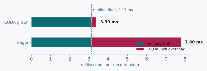
The bus is not slow. The bus is bored.
So the first candidate goes. The bus is not slow. The bus is idle, waiting for a CPU that is 280 function calls behind. Each kernel, once launched, runs at full bandwidth. The problem was never inside any of them. The problem is the gaps between them.
11.4 What This Rules Out
This rules out an entire category of fix, and it is the category everybody reaches for first.
Every kernel in that forward pass could be made twice as fast and the token would still carry 4.67 ms of CPU time, because the CPU work happens between the kernels, not inside them. Optimizing a kernel that is already bandwidth-saturated, in a step where sixty percent of the wall clock is dispatch, is a week spent on the other forty.
It also rules out more bandwidth. A card at 760 GB/s halves the 3.13 ms and leaves the 4.67 alone, taking 7.80 down to 6.23. You would have doubled the most expensive component in the machine for a twenty percent improvement, and the profiler would still show a bus at forty percent utilization, except now it would be at twenty.
What survives is an observation about repetition. That sequence of 280 launches is the same every single token. Same kernels. Same order. Same shapes. Same buffers. We are paying a CPU to make an identical set of decisions several hundred times a second, and it makes them correctly every time, and none of them were ever in doubt.
That is a recording problem.
Several hundred times a second, a computer carefully re-derives a conclusion it has never once got wrong.
CUDA graphs let us capture the whole launch sequence once and replay it as a single submission. The host makes one call instead of 280, and the GPU walks the recorded graph itself. The arithmetic does not change at all. The 3.13 ms of memory traffic is still there, still irreducible, still the floor. What goes away is the waiting.
11.5 The Pictorial
One token, drawn as a timeline of who is doing the work:
  eager, 7.80 ms
  CPU   ##  ##  ##  ##  ##  ##  ##  ##  ##  ##  ...  280 dispatches
  GPU     ##  ##  ##  ##  ##  ##  ##  ##  ##  ##
        ^^  ^^  ^^  ^^   bus idle in every gap

  graphed, ~3.4 ms
  CPU   #                                          one replay call
  GPU    ##############################            same kernels, no gaps
The GPU work is identical in both pictures. The only thing we deleted was waiting for permission.
One division, and we never once had to open a kernel. I have had entire weeks go worse than that.
And notice what we did not have to understand to get here. We never opened a kernel. We never looked at an access pattern. We never learned what the attention implementation does with its tiles, and I could not tell you offhand. We computed a floor, found a gap, divided the gap by a count, and the answer named itself.
Challenges
-
The gap arithmetic assumed ~10 GPU operations per transformer layer. Look up or count the actual operations in one layer of a model you have handy, redo the per-launch division, and say whether 17 µs still looks like dispatch or whether something else is hiding in there.
-
CUDA graphs need static shapes, so a server captures one graph per batch size and pads up. Work out the cost of that padding at batch 5 on a system with graphs at 1, 2, 4, 8, and say when the padding waste would exceed the launch overhead it saves.
-
This chapter's model was 0.6B. Redo the floor and the gap for a 7B model on the same card, and say whether launch overhead is a larger or smaller fraction of the token. Then say what that implies about which deployments care most about this fix.
-
Graph replay reuses the same input and output buffers every time. Describe the bug that produces, in a server handling concurrent requests, if the output buffer is handed to the caller directly. Then describe how you would detect it in production, given that it produces plausible text rather than a crash.
Design Note: The Floor Test Runs in Both Directions
Chapter 1 introduced the floor test as a fraud detector. Compute the fastest the work could possibly go. Measure faster than that. Now you know something you believed was happening did not happen, and a 4 KB write that returns in 200 nanoseconds never reached the disk.
This chapter is the same instrument held upside down, and I have come to think it is the more useful orientation.
Compute the floor, measure well above it, and you have found work you were not modelling. Not a slow component. An unmodelled one. That distinction matters enormously, because it redirects the entire search. A slow component means go profile it and optimize it. An unmodelled component means your picture of the machine is missing a participant, and no amount of profiling the parts you already know about will introduce you to somebody you did not know was in the room.
Both directions share one requirement, and it is the same requirement as chapter 1's design note. You have to compute the floor before you measure. A floor derived afterwards has an unfortunate habit of landing suspiciously close to whatever you happened to observe, and you will never catch yourself doing it. Write down bytes ÷ bandwidth first. Then run the thing. Then let the gap be as embarrassing as it wants to be.
Spending the Idle
Five tokens for the price of one, and no asterisk.
Here is a measurement that ought to be impossible.
Take five candidate tokens, produced by something cheap. Hand all five to the 7B model and ask it to check them in a single forward pass. Five times the arithmetic of an ordinary decode step.
Five times the work at the same price. This is the one place in the book where that sentence is not a warning.
It takes the same 7 milliseconds.
Chapter 7 opened this book's second half with a complaint about exactly the resource that just paid for those five tokens. Generating one token from a 7B model on an A100 spends 45 microseconds computing and 7 milliseconds waiting, and the most expensive processor in the building sits 99.4% idle. Five chapters later we have moved an enormous amount of memory around and never once gone back for it.
12.1 Candidates and the Ratio
That should not be possible, so one of our assumptions is wrong. Either the work we just did was not the work we thought, or it was genuinely free, and only one of those is good news.
The first: the check is not a real check. We are approximating, sampling from something that is not quite the model's true distribution, and the five tokens we get are not the five the model would have produced. Faster and slightly wrong is an old trade, and usually a bad one.
The second: the arithmetic was free, because we had already paid for it and were not using it.
The ratio worth naming is 156 to 1, and we computed it back in chapter 7. If the second is right, then this is not a clever trick at all. It is the natural consequence of standing two orders of magnitude to the left of the ridge, and the only surprising thing is that it took the field until 2023 to go and spend the change.
12.2 The Axioms
Everything we need is already on the table from chapter 7, which is a good sign for a final chapter.
| Quantity | Value |
|---|---|
| Weight bytes read per forward pass | 14 GB, independent of token count |
| FLOPs per token of work | ~14 GFLOP |
| A100 ridge point | ~156 FLOP/byte |
| Memory time for one pass | ~7 ms |
| Compute time per token of work | ~45 µs |
That first row carries the chapter, so let me say it in words too. A forward pass over K tokens reads the weights exactly once, in precisely the way a forward pass over one token does, because the weights have no idea how many tokens are passing through them.
The weights have no idea how many tokens are passing through them, and knowing would not help them in the slightest.
Which is the same fact chapter 7 used to justify batching, applied along a different axis. Batching puts K different sequences through one weight read. This puts K consecutive tokens of one sequence through it.
12.3 Doing the Division
Then the comparison is two lines of arithmetic, and the second one is just the first with a bigger numerator. Same bytes read, five times the operations:
generate 1 token   :  14 GB read,  14 GFLOP  →   1 FLOP/byte
verify 5 tokens    :  14 GB read,  70 GFLOP  →   5 FLOP/byte

ridge point        :                            156 FLOP/byte
Both sit far to the left of the ridge. So both are memory-bound. So both cost exactly what the memory costs:
memory time, either case  :  14 GB ÷ 2 TB/s   =  7.0 ms
compute time, generate 1  :  14 GFLOP ÷ 312 TFLOP/s  =   45 µs
compute time, verify 5    :  70 GFLOP ÷ 312 TFLOP/s  =  225 µs
Doing five times the arithmetic for free is the closest thing to a free lunch in this book, and it took the field until 2023 to order it.
The compute grew by a hundred and eighty microseconds, against a seven millisecond wait. We went from 99.4% idle to 96.8% idle and the wall clock did not move, because at 5 FLOP/byte we are still thirty-one times short of the ridge.
Chapter 7 told us extra compute below the ridge buys nothing. Read that sentence the other way round and it says extra compute below the ridge costs nothing, and that is the whole chapter.
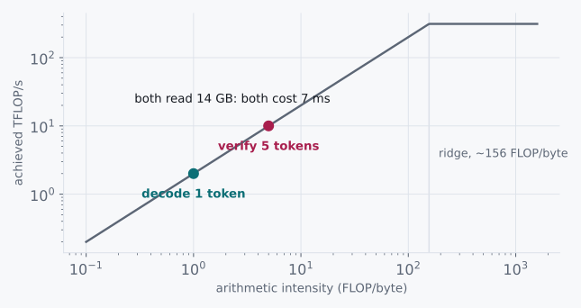
12.4 What This Rules Out
That leaves candidate one, and it is the interesting one to set aside, because the mechanism that does it is genuinely surprising.
The naive way to use five proposed tokens is to accept the ones that match what the model would have picked and stop at the first that does not. Under greedy decoding that is already exactly right. Under sampling it is subtly wrong, because "matches the most likely token" is not the same thing as "drawn from the model's distribution," and a system that quietly sharpens its own sampling is precisely the quality-for-speed trade we were trying to avoid.
Modified rejection sampling repairs it, and here is the whole of it.
Let q be the cheap proposer's distribution and p the real model's. For each proposed token t, accept it with probability min(1, p(t) ÷ q(t)). On rejection, draw the replacement not from p, but from the normalized residual max(0, p − q), and stop there.
That residual is the part that makes it exact, and it is worth understanding rather than memorizing. Accepting at min(1, p/q) alone under-samples the tokens the proposer thought unlikely. Sampling rejections from p − q puts back exactly the mass that step removed. Not approximately. Exactly.
The tokens that come out are distributed according to p. Not close to p. Not p within a tolerance. p.
Lossless and merely-fast produce text that reads exactly alike. Only one of them survives a statistician.
If you only remember one line of algebra from this chapter, make it that subtraction. It is the difference between a technique that is lossless and one that is merely fast, and you cannot tell them apart by reading the output.
So a bad proposer costs speed and never quality. That is a rare shape for a trade-off and worth stating plainly: the failure mode of speculative decoding is that it stops helping.
It also rules out reaching for a large K. If each token is accepted with probability a, then the expected yield of one target pass is one guaranteed token plus the accepted run:
expected tokens per pass  =  1 + a + a² + ... + a^K

at a = 0.7:   K=4 → 2.77      K=8 → 3.19      K=16 → 3.32
Eight consecutive correct guesses is an optimistic afternoon, and 0.7 to the eighth power agrees.
Doubling K from 4 to 8 buys 0.42 tokens, because reaching the eighth proposal requires eight consecutive acceptances, and 0.7 to the eighth is a small number. Past K of about four to eight you are paying draft cost for tokens you will throw away, and eventually paying enough of it to matter even down here below the ridge.
12.5 The Pictorial
Where the proposals come from is almost an afterthought, which I take as the best evidence that this idea is really about the ridge and not about owning a second model.
  n-gram proposer, no model at all:

    context:  ... def fibonacci(n):  if n < 2:  return n   def fib
    search backwards for "def fib" ---^                    ^-- match
    propose what followed last time:  onacci(n):  if n < 2:

  target model verifies all five in one 7 ms pass
  accepts the longest correct prefix, corrects the first miss
For code, for structured output, for anything that quotes its own prompt back, that costs nothing and hits often. A small draft model does better on prose and costs a fraction of a pass. Either way the expensive model runs once and returns several tokens, and the idle compute from chapter 7 is what pays for all of it.
Challenges
-
Verification at K=5 sits at 5 FLOP/byte. Speculation and batching compose: a server running batch 32 with K=5 verification is at some intensity you can compute. Work it out, compare it to the ridge, and say whether the two techniques are still free when used together.
-
Derive the expected-tokens-per-pass formula in 12.4 from the acceptance probability a, rather than taking it on trust. Then find the K that maximizes tokens per pass once you charge the draft model at 5% of a target pass per proposed token.
-
Acceptance rate a is not a constant. Predict whether a is higher when the model is generating code or generating poetry, justify it in terms of the target's output distribution, and say what that implies about advertising a single speedup number for this feature.
-
Chapters 7 through 12 give four ways to move throughput: batch, page the cache, delete launch overhead, and speculate. A serving system has finite engineering time. Order them for a deployment whose requests average 30 output tokens and arrive 4 per second, and justify the order with arithmetic rather than preference. (Nothing above answers this; the arrival rate changes which wall you are against.)
Design Note: The Idle Was the Budget
Chapter 7 computed 99.4% idle and treated it as an indictment. It read like waste. Like something a better engineer would have prevented. The natural response was to go looking for the mistake that caused it, and I sent you looking, and there was no mistake.
Six chapters later the same number is a budget.
The GPU is idle because arithmetic intensity is far below the ridge, and that is not a defect waiting to be repaired. It is a resource sitting unspent. Speculative decoding is the first technique in this book that treats it that way. It does five tokens' worth of arithmetic to produce, on average, fewer than three useful tokens. It throws the rest away. And it comes out ahead, because the arithmetic was never the scarce thing.
Which is the argument the whole book has been making, arriving at last in a form specific enough to be uncomfortable. Every chapter here has been about finding the one quantity that is genuinely scarce and declining to optimize the others. In chapter 3 it was the fsync round trip and not the bytes. In chapter 8 it was memory capacity and not compute. Here it is bandwidth, and the correct response to a scarce resource is to spend the abundant ones freely, including on work you fully expect to discard.
The uncomfortable part is that this reverses what good engineering feels like. Doing arithmetic you know will be thrown away, deliberately, at a ratio of five to three, offends an instinct most of us have been rewarded for having our entire careers. And that instinct is correct, whenever compute is scarce. It is precisely wrong here. Telling those two situations apart is what the ratio in chapter 7 was always for.
That is where this book stops deriving and the course starts building. Twenty stages, each gated on a measurement rather than on your code merely running: the naive loop, the KV cache, the roofline you just read about, static and then continuous batching, the block allocator, paged attention in PyTorch and then in Triton, prefix caching, the scheduler, chunked prefill, CUDA graphs, the sampler, the detokenizer, the server, and the rejection sampler from this chapter.
The chapters tell you which number matters and why. The stages will not let you past until your version of it moves.
The Course
Twenty stages, and not one of them passes because the code ran.
Chapter 12 ends by saying that this is where the book stops deriving and vllm-from-scratch starts building. This page is that repository's map: what the twenty stages are, in what order, and which number each one will not let you past until it moves.
The split is worth being precise about, because it is the reason these are two things instead of one longer book. A chapter's job is to find the single quantity that is genuinely scarce and show you the arithmetic that makes it scarce. It has done its job when you can predict the number. The course does not care whether you can predict continuous batching's win. It cares whether your continuous batching used under 60% of the forward passes your static batching needed, on your card, this afternoon.
There are 229 checks across the twenty stages, and most of them assert a
measurement rather than a behaviour. ./vc submit refuses to advance
while anything is red, so there is no way to skip a stage by being
impatient with it. (222 checks if you take the JAX route, which is two
sections down, and which is the same twenty stages.)
That refusal is the whole product. Anybody can read twenty descriptions of PagedAttention. Rather fewer people have had a test inform them that their page table is perfectly correct and four times slower than the contiguous cache it replaced, which is the actual experience of writing one, and which is stage 7.
Start without installing anything
The honest problem with handing somebody a repository is that they have to set it up first, and the setup here is a virtual environment, a couple of gigabytes of PyTorch, and a model download, on a machine that might not have a GPU in it at all. That is a great deal of friction to pay before you know whether you want the thing.
So there is a notebook. It clones the course onto a free Colab T4, runs the setup, and leaves you at stage 1's guide, and it costs you a browser tab.

It also puts the GPU stages within reach of a machine that cannot run them. Stage 8 is a Triton kernel, stage 12 captures CUDA graphs, stage 18 wants FP8: on a laptop with integrated graphics those are three stages you can read and not do. On a T4 they run.
One caveat, and it is a real one. A Colab runtime is temporary. Your
progress lives in .progress.json inside that container, and when the
session resets it goes, along with everything you wrote. That is fine
for working through the first arc and finding out whether you care. It
is not where you would do all twenty. The notebook's last cell pushes
your work to your own fork, and past about stage 5 you should take it up
on that.
Or run it on your own machine
gh repo fork Venugopalan2610/vllm-from-scratch --clone
cd vllm-from-scratch
./setup.sh        # python 3.12 venv, torch, and the model. once, ~5 min.
./setup.sh --jax  # and JAX too, if you want the second track. +400 MB.
Fork rather than clone, because ./vc submit commits your work and you
will want somewhere to push it.
No GPU is not fatal. Setup still works and about half the stages still run, because the allocator, the scheduler, the prefix cache, the metrics, the speculative sampler and the guided decoder are pure logic and were deliberately written to be testable without a card.
The loop
./vc              # where am I?
./vc guide        # what to build, and why it comes here and not earlier
                  # ... go and edit the file it names ...
./vc test         # run the checks. as often as you like.
./vc submit       # all green? banked, committed, next stage opens
./vc submit commits only app/, which is your work, and prints the
next stage's guide. There is also ./vc math if you want the arithmetic
for your own card rather than the book's A100, and ./vc peek if you
are genuinely stuck and would rather read the answer than abandon the
ladder. Reading the answer is a worse outcome than working it out and a
much better one than quitting.
Two ladders, one physics
Here is a question I did not expect to have to answer, and the answer turned out to be worth more than the question. Does any of this depend on PyTorch?
It had better not. The whole book is an argument from one physical fact, that fetching a weight from HBM costs far more than the arithmetic you then do with it, and silicon does not care which Python library you type at it. But claiming that and demonstrating it are different activities. So the course runs on two backends now.
./vc backend jax      # switch tracks. progress is banked per track.
./vc test 8 --jax     # or just one command on the other, without switching
Twenty stages either way. Eleven of them get a JAX twin, so you edit
app/j08_paged_pallas.py where the other track edits
app/s08_paged_triton.py. The remaining nine are not twins. They are
the same file.
Read that again, because it is the finding, and I did not go looking for it. The block allocator, the prefix cache, the scheduler, chunked prefill, the incremental detokenizer, the async server, the metrics, the speculative sampler and the guided decoder were never ported, because there is nothing in them to port. Not one of them contains a tensor operation worth the name. Nearly half of an inference engine is refcounts, free lists, three queues and a hash table, and it would look much the same if you wrote it in Go.
Allow yourself a moment of disappointment about that, and then notice that it is good news twice over. The hard part is not the framework. And the part you were afraid of, the kernel, is a minority of the work.
Where they do diverge, they diverge from one cause
XLA compiles a program for exact shapes. Torch dispatches a kernel per operation, at runtime, from whatever shape the tensor happens to have. So a KV cache that grows by one token per step, which is the obvious design and the one the torch track uses, is a brand new program every step. Seconds of compiler. Per token.
You fix it by refusing to change the shape: preallocate the cache to its maximum and write into it. That is one sentence, and it moves four stages sideways.
Stage 2 hands you back the bookkeeping torch was quietly doing on your
behalf, because now cache_len is yours to carry. Stage 4 right-pads
where the other track left-pads, since the padding belongs where the
generated tokens are about to land, and then you have to tell the model
which row's logits to read. Get that wrong and the short prompts in your
batch produce fluent continuations of the padding, which is a much worse
failure than an error, because it looks like text.
Stage 5 is the one I would send somebody to. When a sequence finishes you cannot shrink the batch, because the batch dimension is the compilation. So the batch becomes a fixed table of slots. Finishing frees one, admitting fills one, and nothing is copied or re-indexed at all. That is a page table with one page per sequence, and you have arrived at it a whole arc before the course meant to introduce the idea.
There is a sting in it. A step costs the same whether one slot is busy or eight, so continuous batching cannot possibly show up as a faster step. It shows up as useful tokens per forward pass, and occupancy becomes the entire game. The idea from The Slot That Waited survives intact. The number you measure it with does not.
The stage that convinced me
Stage 12, on the torch track, captures CUDA graphs. You know why from Below the Floor: a decode step at batch 1 is about a millisecond of GPU work and about a millisecond of Python issuing kernel launches, and the graph deletes the second millisecond.
None of that is true in JAX. XLA already fused the step into one program. There is one launch. The Python is gone.
And stage 12 on the JAX track does exactly the same thing anyway. Pick a handful of batch sizes, compile ahead of time for each, pad up to the nearest one. The same fix, to the letter, for a completely unrelated disease: not launch overhead but compilation, which is what you pay every time a batch size you have not seen before walks in the door.
That is the strongest evidence in the repository that bucketing is not a CUDA trick. It is what you do whenever preparing to run the work has started to cost more than the work.
Two places JAX is simply better, and one where it is not
Stage 8 is Pallas rather than Triton, and the online softmax is, line for line, the same idea. What changes is the indirection. Pallas gives you a BlockSpec that declares which tile of an array each program sees, which is a lovely abstraction right until the tile you need depends on a page table you have not read yet. So the block table lookup moves inside the kernel, with an index you compute there. The one thing the abstraction cannot do for you is precisely the thing PagedAttention is.
Stage 20 stops being a simulation, and I am slightly embarrassed by how
much better it gets. The torch track shards weights in a Python loop and
then spawns two gloo processes to prove a collective works. JAX simply
hands you devices. shard_map over a mesh, column-parallel and then
row-parallel, and the psum is a real all-reduce, so "exactly one
collective per block" stops being a claim in prose and becomes something
the check counts in the compiled HLO.
Now the honest one. Decode on the JAX track gets slower as the cache gets bigger, and it should not. The preallocated buffer is rewritten functionally, per layer, inside the scan, so you pay for the ceiling you chose rather than the context you actually hold. Roughly 1.3x going from a 128-slot cache to a 1024-slot one, where the torch track is nearly flat. Buffer donation does not rescue it, because the copy is inside the scan where the donation cannot reach.
Stage 3 says so, in the test, with the number, rather than quietly choosing a friendlier measurement. What actually fixes it is making the buffer granular so that a step only touches the blocks it needs, which is PagedAttention, which is the next arc. The JAX track gives you a reason to want stages 6 through 9 before you have finished stage 3. I would not have been clever enough to design that on purpose.
Which chapter derives which stage
Six of the twelve chapters have a stage that builds what they derived. Those are the ones where reading and building are the same activity done twice, and doing both in that order is the intended path.
| Chapter | Stages |
|---|---|
| The Ridge | 01–03, the naive loop and the roofline |
| The Cache That Ate the Batch | 02, KV bytes per token |
| The Slot That Waited | 04–05, static then continuous batching |
| A Page Table for Tokens | 06–09, blocks, paged attention, prefix cache |
| Below the Floor | 03 and 12, the gap and CUDA graphs |
| Spending the Idle | 17, the n-gram proposer and rejection sampler |
The rest have no chapter deriving them, and I would rather say so than pretend the coverage is complete. Stages 10, 11, 13 through 16 and 18 through 20 build the scheduler, chunked prefill, the sampler, the detokenizer, the server, quantization, guided decoding and tensor parallelism. They are good stages. They are simply ahead of the prose.
The ladder
Seven arcs. The order is not the order a textbook would choose: it is roughly the order the ideas were actually discovered, which means every stage exists because the previous one broke in a specific way, and the guide for each one opens by telling you what that way was.
The pips are how hard the code is, not how hard the idea is. Stage 3 is two stars and is the most important thing in the course.
A0 · The Naive Loop
Build the slow thing first, and measure it, so every later win is a number.
01 · Greedy decode, no cache [*....]
A transformer forward pass is a pure function of the whole prefix. Generating N tokens naively costs O(N^2) attention work because you recompute every previous token's K and V on every single step.
02 · The KV cache [**...]
K and V for a token never change once computed. Cache them and each decode step becomes a single-token forward pass: O(N) total. This is also the moment memory becomes your enemy instead of compute.
03 · Prefill vs decode: two different machines [**...]
Prefill is compute-bound (big GEMMs, high arithmetic intensity). Decode is memory-bandwidth-bound (batch size 1 means every weight is read from HBM to produce one token). They want opposite optimizations. This is THE fact that explains every design decision downstream.
A1 · Batching
Decode is bandwidth-bound, so extra sequences are nearly free. Exploit that.
04 · Static batching with padding [**...]
Batching amortizes the weight read across sequences: 8x the tokens for almost 1x the time. But a static batch runs until its SLOWEST member finishes, and short sequences sit padded and idle, burning the slot.
05 · Continuous batching (iteration-level scheduling) [***..]
Schedule per ITERATION, not per request. When a sequence emits EOS, evict it that same step and admit a waiting one into its slot. From Orca (OSDI '22). Typically 2-4x over static batching on real traffic, and it is the single largest throughput win in this entire repo.
A2 · PagedAttention
The idea vLLM is named after. Virtual memory, applied to the KV cache.
06 · Blocks, block tables, free list [***..]
Contiguous per-sequence caches force you to pre-allocate for max_len, so real serving wastes 60-80% of KV memory to internal fragmentation and reservation. Chop the cache into fixed 16-token blocks, hand them out on demand, and keep a per-sequence block table (a page table). Waste drops to under one block per sequence.
07 · Attention that reads through the page table [****.]
The kernel must gather K/V from scattered blocks instead of striding a contiguous tensor. Do it in PyTorch first (index_select + SDPA) to get it CORRECT, then keep that as the reference oracle forever.
08 · The same thing, fast [*****]
One program per (sequence, head, block); stream K/V tiles through SRAM; online-softmax so you never materialize the full score row. Decode attention is bandwidth-bound, so your kernel's job is coalesced reads.
09 · Copy-on-write and automatic prefix caching [****.]
Block tables make sharing trivial: two sequences can point at the same physical block. Refcount them, copy-on-write when one diverges. Then hash block contents and reuse across REQUESTS: a shared system prompt gets prefilled once for everybody. This is why APC feels like cheating.
A3 · The Scheduler
You have finite KV memory and infinite requests. Decide who runs.
10 · Waiting / running / swapped, and preemption [****.]
Sequences grow one block at a time, so the batch you admitted can run out of memory mid-decode. You need preemption: either SWAP blocks to CPU or DROP them and recompute later. Recompute usually wins, because prefill is fast and PCIe is not.
11 · Chunked prefill and mixed batches [****.]
One 8000-token prefill stalls every decoding sequence for a whole step, wrecking inter-token latency for everyone. Split prefill into chunks and co-schedule chunks with decodes in the SAME batch. From Sarathi-Serve. This is the throughput/latency dial in every modern serving stack.
A4 · Making It Actually Fast
Everything left is overhead removal.
12 · CUDA graphs for the decode step [****.]
At batch 1 a decode step is ~1ms of GPU work and can be ~1ms of Python and kernel-launch overhead. Capture the whole step as a graph and replay it. Requires static shapes, so you capture at bucketed batch sizes and pad up to the nearest bucket.
13 · A real batched sampler [***..]
Every request has its own temperature, top-k, top-p, penalties, and seed, and they all must be applied in ONE vectorized pass over the batch. The naive per-request Python loop silently becomes your bottleneck once the kernels are fast.
14 · Incremental detokenization and stop conditions [***..]
You cannot decode tokens independently: BPE pieces, multi-byte UTF-8, and leading-space rules mean naive streaming emits mojibake and doubled spaces. Stop STRINGS can also straddle a token boundary, so you must buffer. Boring, and the source of most user-visible bugs in real servers.
A5 · The Server
Turn the engine into something you can curl.
15 · Async engine + OpenAI-compatible API [***..]
The engine loop must never block on HTTP, and HTTP must never block on the GPU. One process runs step() forever; requests are futures/queues fed into it. Real vLLM V1 pushes this further, into a separate EngineCore process, so Python overhead on the API side cannot stall the GPU.
16 · The metrics that matter [**...]
TTFT, TPOT/ITL, throughput, queue wait, KV utilization, preemption rate. If you cannot see KV utilization and preemption count, you cannot tune anything, and you will misdiagnose every performance problem you hit.
A6 · Modern vLLM
Optional, but this is where the field currently is.
17 · Draft, verify, reject [*****]
Decode is bandwidth-bound, so verifying K tokens costs about the same as generating 1. Propose K with something cheap (n-gram lookup or a tiny model), verify in one pass, accept the longest correct prefix. Modified rejection sampling keeps the output distribution EXACTLY unchanged.
18 · Weight-only quantization [****.]
Decode reads every weight per token, so halving weight bytes nearly halves decode time. INT8/FP8 weight-only with per-channel scales, dequantized in the kernel epilogue. Also quantize the KV cache: it is the other big reader.
19 · Constrained output via logit masking [****.]
Compile a grammar/JSON schema to an FSM over token ids, and mask illegal logits each step. The hard parts are tokenizer alignment and doing the mask build off the critical path so it does not stall the GPU.
20 · Tensor parallelism (simulated on one GPU) [*****]
Shard attention heads and MLP columns across ranks; one all-reduce per layer. You have one GPU, so run 2 ranks on it with NCCL to get the collectives and the sharding logic right. The lesson is where the communication lands, not the speedup.
Rules Index
The page to open at 11pm. Each rule links back to the derivation that earned it. If you can rebuild the argument from the rule alone, you're done; if not, follow the link.
I. The Method
- Ratio triage: sort next questions by the spread between their possible answers. >10×: ask now. <2×: it's a detail.
- The floor test: when a measurement beats your theoretical floor, the work didn't happen.
- Match the instrument to the ratio: 1000× apart, wall clock. 1.5× apart, counters.
II. Durability
- Test the failure you claim to survive: a crash test that can't reach the layer your data lives in has proven nothing about that layer.
- Buy durability at boundaries, not by the record: fsync cost is dominated by the round trip, not the bytes. Pay it once per boundary, never once per write.
- fsync failure is not retryable: once fsync errors, the page behind it is already gone. Recover from an independent durable source, don't retry the same call.
- Let the barrier set its own batch size: close the batch when the in-flight fsync returns, not when a counter hits a constant.
- Checksum every record; seed the register nonzero: torn writes pass structural checks by accident. Only arithmetic over the content finds where the truth stops.
III. Accelerators
- Check arithmetic intensity before adding FLOPs: below the ridge point, more compute buys nothing. The wait is on bytes, not operations.
- Size your batch from the KV budget, not a guess: before blaming scheduling for a batch ceiling, check bytes-per-token × context length × concurrency against free memory.
IV. Building the Answer
- Release the slot when the sequence ends, not when the batch does: schedule per forward pass, not per request. A finished sequence leaves on the step it finishes; a waiting one takes its place.
- Page the cache; reserve for the token you have: when a per-client allocation grows unpredictably toward a large ceiling, allocate fixed-size blocks behind an indirection table.
- A workload that misses its own roofline floor is not yet bound by what you think: when a memory-bound workload takes longer than bytes ÷ bandwidth, the extra time is on the host. Count launches before optimizing kernels.
- Below the ridge, spend compute on work that might be wasted: idle compute does not accrue. Far under the ridge point, speculative work is free even when most of it is discarded.
Challenges
Every question in the book, stripped of context and answers. Revision by retrieval, not rereading.
1 · Twenty-Five Microseconds
- A 4 KB write measures 900 ns. Which layer, and which floor decided it?
- A service acks after
write()returns. Which failure loses acked data, and which doesn't? - Someone claims a 3× speedup. First question, and what would make you
reach for
perf? - Derive the max durable-write rate for one
fsyncper request, then explain why real databases beat it.
2 · The Ladder
- A crash harness uses
kill -9and a cleanrebootbetween runs. Which row does that validate, and which row does it still miss? - Does
echo b > /proc/sysrq-triggersit closer tokill -9or to a real power cut? Justify it from what each one destroys. - An NVMe spec sheet doesn't mention power-loss protection. What experiment tells you whether it has it, without opening the case?
- Redraw the power-loss column as a function of shared-UPS failure rate. At what point does "no PLP on the drive" stop being a real risk?
3 · The Barrier
- Batching 100 records behind one
fsync: best-case throughput gain, and what makes the real gain fall short of it? - When does
fdatasyncnot actually save you a barrier crossing? - Two threads
fsyncthe same file near-simultaneously. Does the second call cost a full barrier or something cheaper, and how would you find out? - Does
O_DIRECTmakefsyncunnecessary? Name the specific claimfsyncmakes that a direct write alone doesn't.
4 · Write-Ahead
- Why does calling
fsyncin a retry loop until it "succeeds three times" not fix the terminal-error problem? - WAL fsync succeeds, ACK is sent, then the process crashes before data pages are written. Where does correct final state come from?
- What changes about worst-case commit latency if the ACK moves to after the data-page write instead of right after the WAL fsync?
full_page_writesdoubles WAL volume after every checkpoint. Reduce that cost without weakening the torn-page guarantee.
5 · Group Commit
- At exactly one arrival per fsync-latency window, what does adaptive batching's average batch size converge to, versus fixed N=2?
- Load spikes past what a 200 µs floor can drain. Does the floor still help, or start hurting?
- Two writers share one log file. What has to be true about their fsync coordination for adaptive batching to stay correct?
- Redo the arithmetic for two durability tiers: some callers need the fsync ack, some are fine off the page cache. One batch, or two?
6 · Where the Truth Stops
- Record 3's CRC matches, but record 2 before it was torn and truncated the file mid-record. Does record 3's match mean anything?
- Upgrading 16-bit → 32-bit checksum: new odds of undetected corruption, and at what write rate would you expect one over a year?
- CRC isn't cryptographically secure. Under what threat model does that matter for crash recovery, and under what model doesn't it?
- Design a scheme where a torn checksum trailer still gets the record correctly rejected. What has to be true about where it lives?
7 · The Ridge
- What batch size reaches ~156 FLOP/byte, and what has to be true about traffic for that batch to fill without unacceptable latency?
- A 13B model roughly doubles both weight bytes and FLOPs per token. Does its ridge-crossing batch size move, and which way?
- fp16 → int8 halves bytes without changing FLOPs much. Recompute arithmetic intensity at batch 1. Closer to the ridge or not?
- Redo the FLOP/byte arithmetic for a 2048-token prefill pass (matrix-matrix, not matrix-vector). Compute-bound or memory-bound?
8 · The Cache That Ate the Batch
- GQA with group size 8 divides KV cache per token by ~8. Recompute the batch ceiling and check it against the ridge's target of ~156.
- Design a memory-accounting scheme for mixed-length sequences that doesn't pad everyone to the max length.
- int8 KV quantization halves bytes/token. Does it move the ridge point, the batch ceiling, or both?
- Estimate whether a 70B model's KV-cache-per-token is closer to 5× or 10× the 7B figure, and redo the 80 GB budget.
9 · The Slot That Waited
- The loop evicts finished sequences before the forward pass. What happens if you evict after it, and precisely which token goes missing?
- Admitting a request means splicing its prefilled KV into a batch whose sequences are all at different lengths. What is the copy cost proportional to, and why does that make admission expensive exactly when you want it cheap?
- What output-length distribution still produces low occupancy under iteration-level scheduling, and does it occur in practice?
- Design the admission rule for a request arriving at a full batch, given that you do not know how long it will run.
10 · A Page Table for Tokens
- Average internal fragmentation per sequence at block sizes 1, 16 and 256. What goes wrong at each end? One failure isn't about memory.
- Paging drops the admission cost from 1 GB to one block. Write the admission rule, then find the failure it introduces mid-generation.
- Two sequences share a block by refcount; one writes into it. What must happen, in what order, and what breaks if the refcount is decremented after the copy instead of before?
- Why isn't hashing a block's own tokens enough to recognise a shared prefix, and what else goes into the hash? (The failure is a correctness bug and a privacy bug at once.)
11 · Below the Floor
- Count the real GPU operations in one transformer layer, redo the per-launch division, and say whether 17 µs still looks like dispatch.
- Graphs are captured at batch 1, 2, 4, 8 and padded up. Cost of that padding at batch 5, and when it exceeds the launch overhead it saves.
- Redo the floor and the gap for a 7B model on the same card. Is launch overhead a larger or smaller fraction, and which deployments care?
- Graph replay reuses one output buffer. Describe the bug that causes under concurrency, and how you would detect it given that it produces plausible text rather than a crash.
12 · Spending the Idle
- Batch 32 with K=5 verification sits at what arithmetic intensity? Compare to the ridge and say whether both techniques are still free together.
- Derive expected tokens per pass from the acceptance rate a, then find the K that maximizes it once the draft costs 5% of a target pass per proposed token.
- Is acceptance rate higher for code or for poetry? Justify it from the target's output distribution, and say what that implies about advertising one speedup number.
- Order the four throughput levers (batch, page, delete launch overhead, speculate) for a deployment averaging 30 output tokens at 4 requests/sec, using arithmetic rather than preference.
Experiments
A book that tells you to commit to a number before you measure owes you something to measure with. These are the programs that check the book's own claims, on your hardware, against your filesystem.
They live in experiments/
in the repository.
cd experiments && ./run-labs.sh    # check every claim
cd experiments && ./predict.sh     # commit to a number first
Exit code 0 means every claim in the book that this can reach held on your machine. Nonzero means one did not, and the output names it. Nothing needs root, and each lab cleans up after itself.
They check claims, not numbers
A benchmark prints a number, and you cannot tell a correct run from a broken one. So these assert ratios and exact invariants instead, because those are what survive the change of hardware that absolute latency does not.
A 700 µs fsync and a 100 µs fsync are both ordinary. An fsync that
costs the same as a buffered write means you are not measuring storage
at all, and every conclusion under it is void. That is a claim, so it
is a check: run the labs against a tmpfs and measuring-real-storage
fails loudly rather than quietly reporting that RAM is quick.
Point them at the right filesystem first
This matters more than any other setting. The default is the current
directory, which is usually what you want. But run these against /tmp
on a tmpfs and you are measuring RAM, and every number that comes out
is fiction.
PERFBOOK_DIR=/mnt/nvme ./run-labs.sh
Every experiment prints its kernel, filesystem, device, and whether it detected a hypervisor before it prints a single measurement. If that block does not say what you expected, stop there. The environment is the result; the latency is just a number attached to it.
Part IV has a course rather than a lab
Chapters 9 through 12 derive an inference engine, and deriving it is as far as prose can honestly take you. Building it is too big to be a lab on this page, so it is twenty stages in a repository of its own, and The Course is its map: the whole ladder, which chapter derives which stage, and a notebook that runs the thing on a free GPU without your installing anything.
It is the same contract as the labs here, scaled up. A stage does not pass because the code executes; it passes because continuous batching used under 60% of the forward passes static batching needed, or because your Triton kernel beat your PyTorch one by more than 3x while agreeing with it to 1e-3.
What each one tests
| Lab | Chapter | Claims |
|---|---|---|
02_ladder_survival | The Ladder | 3, exact byte counts |
03_fsync_cost | The Barrier | 3, all ratios |
05_group_commit | Group Commit | 4, ratios, at two arrival rates |
06_crc_zero_seed | Where the Truth Stops | 6, exact, including a CRC-32 known-answer test |
01_write_latency | Twenty-Five Microseconds | timing survey |
Where the data has been, located by survival
02_ladder_survival forks a writer, kills it with SIGKILL at three
moments, and counts what is left:
| killed after | survives | so the bytes were |
|---|---|---|
fwrite | 0 bytes | in the process's own memory, rung 1 |
fwrite + fflush | all of them | in the kernel's page cache, rung 2 |
+ fsync | all of them | rung 2 at least; this test sees no further |
Those counts are identical on every Linux machine. The third row is the instructive one: it passes and proves nothing the second did not. A test that cannot reach rung 3 tells you nothing about rung 3, which is Rule 4, and the lab is a worked example of the mistake that rule warns about.
mincore() and
posix_fadvise(DONTNEED) instead. It was dropped: a control
file written with O_DIRECT, which by definition never
enters the page cache, still reported 100% resident. The probe was
measuring itself. Survival is cruder and correct.
The timing labs will give you different numbers than they gave me, and that is expected. Their claims should still hold, because the claims are ratios. The exact-invariant labs print the same values on every machine, which is what makes them checkable rather than anecdotal.
results.json
Every run appends a manifest recording the git commit, whether the tree was dirty, the compiler, and a hash of each source file, then one object per lab with its environment and every claim's outcome. Send that file rather than a screenshot. It is the difference between "it was fast on my laptop" and a result somebody can argue with.
Your numbers will not match the book's
They are not supposed to. The axioms in these chapters are
order-of-magnitude figures for a class of hardware, and your device is
a specific one. On the machine these were developed on, a consumer NVMe
drive on ext4, fsync costs closer to 700 µs than the 100 µs chapter 3
quotes, because ext4 commits its journal on every sync and the drive
has no power-loss capacitor to acknowledge from.
That gap is not a problem to explain away. It is the exercise. Rule 1 says name the ratio: yours is roughly 7×, and the interesting question is which of those two causes owns most of it.
Method
Percentiles, never the mean. A mean latency averages the number you care about with the number you care about much more. Each experiment reports min, p50, p95, p99, and n.
Warmup iterations, discarded. The first few runs pay for page faults and cold caches that steady state does not.
The clock is measured too. Every run prints its own
clock_gettime overhead. If a result is within an order of magnitude
of that figure, the result is the instrument.
The GPU labs, on a free Colab T4
Chapters 7 and 8 turn on a ratio between a GPU's compute throughput and its memory bandwidth, so checking them needs a GPU. Colab's free tier has one, which puts these within reach of anyone.
They do not trust the datasheet. Vendor peak figures are marketing, and the ridge point is a division of two of them, so the labs measure your card's bandwidth with a large copy, measure its matmul throughput with a large matmul, and divide. The ridge you get is yours.
| Lab | Chapter | Claims |
|---|---|---|
07_roofline | The Ridge | 5, ratios and shapes |
08_kv_cache | The Cache That Ate the Batch | 5, mostly exact |
07 sweeps a batch size from 1 to 256 across a 4096 by 4096 weight
matrix and reports both arithmetic intensity and the fraction of the
card's own peak it reaches. On the laptop card these were built
against, the measured ridge was 183 FLOP/byte, batch 1 landed at
1.0 FLOP/byte and 1.3% of peak, and batch 256 effectively saturated it.
A T4's numbers will be much smaller and every claim will still hold,
because the claims are ratios.
08 checks the 512 KB per token by allocating a real KV cache and
asking CUDA what it cost, rather than trusting the multiplication. It
also measures that Grouped-Query Attention with 8 query heads per KV
head divides that figure by exactly 8.
What is deliberately missing
Chapter 2 wants a power-loss test, and you cannot honestly run one from inside the machine that is losing power. That is the chapter's whole argument, so faking it in software would be worse than leaving it out. It needs a managed PDU or an IPMI power cycle and a second machine to verify from.
Nothing else, for now. Chapter 4's write-ahead argument is checked indirectly by chapters 2 and 3's labs, since it is built on their two results rather than on a measurement of its own.